On an Exact Step Length in Gradient-Based Aerodynamic Shape Optimization


Zienkiewicz Centre for Computational Engineering, College of Engineering, SwanseaUniversity, Bay Campus, Fabian Way, Crymlyn Burrows, Swansea SA1 8EN, UK
*
Author to whom correspondence should be addressed.
Fluids 2020, 5(2), 70; https://doi.org/10.3390/fluids5020070
Submission received: 31 March 2020
/
Revised: 4 May 2020
/
Accepted: 9 May 2020
/
Published: 13 May 2020
(This article belongs to the Special Issue Recent Numerical Advances in Fluid Mechanics, Volume II)
Abstract
:This study proposeda novel exact expression for step length (size) in gradient-based aerodynamic shape optimization for an airfoil in steady inviscid transonic flows. The airfoil surfaces were parameterized using Bezier curves. The Bezier curve control points were considered as design variables and the finite-difference method was used to compute the gradient of the objective function (drag-to-lift ratio) with respect to the design variables. An exact explicit expression was derived for the step length in gradient-based shape optimization problems. It was shown that the derived step length was independent of the method used for calculating the gradient (adjoint method, finite-difference method, etc.). The obtained results reveal the accuracy of the derived step length.
1. Introduction
The combination of computational fluid dynamics with numerical optimization algorithms has become a numerical tool used to predict the optimal shape for aerodynamic configurations, such as airfoils. During the last few decades, aerodynamic shape optimization has been an important area of research and great advances have been made due to the rapid progress in the development of high-performance computers and computational algorithms. The traditional “trial and error” approach used to design aerodynamic configurations is based on wind-tunnel testing. Nowadays, the high cost associated with wind-tunnel testing of real aerodynamic models is significantly reduced using numerical shape optimization. Instead of costly experiments of a whole range of aerodynamic configurations, only the optimal shape predicted bythe computational analysis is tested in the wind tunnel. When validated this way, the optimal design may be used in the development of the final aerodynamic configuration. To make this approach viable, shape optimization algorithms for aerodynamic configurations must be as efficient as possible.
Among the factors involved in aerodynamic shape optimization are the type of flow regime (subsonic, transonic, supersonic, hypersonic), the governing equations (Laplace, Euler, Navier–Stokes), the grid used to mesh the flow domain (structured, unstructured, if structured: O-type, C-type, H-type, or hybrid), the design variables and the angle of attack, the method of discretization of the governing equations (finite element method (FEM), finite difference method (FDM), finite volume method (FVM)), the optimization method (Newton and quasi-Newton methods, conjugate gradient, genetic algorithm, etc.), the shape sensitivity analysis (finite-difference method, adjoint method, automatic differentiation, etc.), the aerodynamic body to be optimized(airfoil, wing, fuselage, blades, etc.), the objective function definition, the body parameterization method, and the imposed constraints (geometrical, etc.).
In Hicks and coworkers [1,2], computational fluid dynamics was combined with numerical optimization to predict theoptimal shape design for airfoils and wings. In Hicks et al. [1], the drag on nonlifting symmetric transonic airfoils in an inviscid flow is minimized under geometric constraints. The numerical optimization method is based on feasible directions and the inviscid flow is governed by the transonic, small-disturbance equation. In Hicks et al. [2], the optimal shape design of a wing is studied. The problems of drag minimization and lift-to-drag ratio maximization are addressed bysolving the three-dimensional full potential equation coupled with the conjugate gradient method. The first use of adjoint equations for optimal design problems in fluid dynamics is presented inPironneau [3] and for aerodynamic shape optimization problems governed by the full potential and the Euler equations arepresented in Jameson and coworkers [4,5,6,7]. The application of the adjoint method to aerodynamic shape optimization has been the subject of intensive research during the past few decades [8,9,10,11,12]. The optimal shape design in fluid mechanics and aerodynamics using different methods is thoroughly studied inMohammadi and Pironneau [13] and an excellent study on the coupling of computational fluid dynamics and optimization methods is given inThevenin and Janiga [14]. A thorough examination of various aerodynamic optimization methods is given inSkinner and Zare-Behtash [15]. An extensive study on the mathematical aspects of the discrete adjoint method is presented in Giles and coworkers [16,17]. InElliott and Peraire [18], the discrete adjoint method is used to calculate the gradient of the objective function with respect to design variables in airfoil and wing inverse design problems governed by the Euler equations using unstructured meshes. It is shown that the computation of the gradient of the objective function using the adjoint method is independent of thenumber of design variables. In Nemec and Zingg [19], a Newton–Krylov algorithm is applied to the discrete adjoint and the discrete flow-sensitivity approaches to calculate the gradient of the objective function in some two-dimensional aerodynamic shape optimization problems governed by the Navier–Stokes equations. The design problems considered include an inverse design, maximization of the lift-to-drag ratio, lift-constrained drag minimization, and lift enhancement. In Anderson and Venkatakrishnan [20], the continuous adjoint method is formulated and applied for aerodynamic shape optimization problems governed by the Euler and Navier–Stokes equations using unstructured grids for different objective functions, such as drag minimization, lift maximization, and an inverse design (based on a pressure distribution).
By increasing the number of design variables in large-scale aerodynamic shape optimization problems, the most efficient method forcalculating the involved gradients is to combine gradient-based optimization methods, such as steepest-descent, conjugate-gradient, or quasi-Newton method, with the adjoint method. In the gradient-based optimization methods, the iterative process used to update the solution is based on the calculation of two variables: (1) the direction of descent and (2) the step length (a positive scalar). The former, which may be obtained from the calculation of the gradient of the underlying objective function, specifies the direction along which the value of the objective function is reduced, while the latter determines the distance that the updated solution should move in the direction of descent to substantially minimize the objective function. The success of a gradient-based optimization method depends on effective choices of both the direction of descent and the step length [21]. In aerodynamic shape optimization problems, the gradient of the objective function may be determined usingthe finite-difference method or the adjoint method. The step length is calculated usingline search or trust-region methods. If the objective function to be minimized can be expressed as a polynomial function, one can find an exact step length; otherwise, an inexact step length may be obtained usingthe line search or trust-region methods, and it is chosen in such a way that some conditions, such as the Wolfe conditions, are satisfied [21]. To the best of our knowledge, in aerodynamic shape optimization problems, there exists no exact expression for the step length. In this study, an exact step length is developed for the first time for unconstrained minimization problems in aerodynamic shape optimization, such as drag and drag-to-lift ratio minimization problems.
2. Governing Equations
The steady inviscid transonic flows considered here are governed by the Euler equations. In this study, these equations were solved using the ANSYS Fluent v19.2 software (ANSYS, Inc., Canonsburg, PA, USA) to obtain the airfoil surface pressure distribution needed to calculate the sensitivity coefficients using the finitedifference method.
Airfoil Parameterization
In this study, Bezier curves (BezierAirfoil: A MATLAB code for generating an airfoil shape using Bezier curve-V2. DOI: 10.13140/RG.2.2.30002.56000) were used to parameterize the airfoil surfaces.
Bezier curve: The mathematical definition of a Bezier curve is as follows:
where
is the Bernstein basis polynomial of degree , , and . and are the - and - coordinates of the predetermined data points on the airfoil surface. By convention: and . The order of a Bezier curve is equal to (the number of the control points).
The parametric Bezier curve of interest here was of order 11 (because it can successfully generate a large number of airfoil shapes with a high degree of accuracy) and is given as follows:
In this study, the -coordinates of airfoil nodes were considered constant during the optimization, . Therefore, for the predetermined -coordinate of the airfoil nodes, we could write:
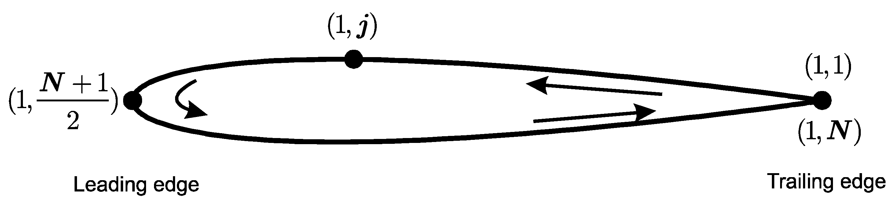
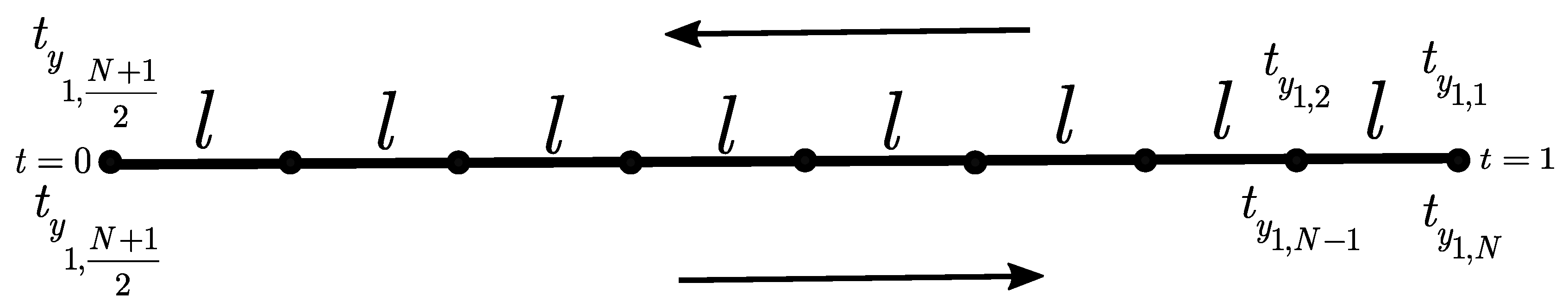
Therefore, the Bezier control points could be obtained at the first iteration for the predetermined -coordinate of the initial airfoil. Two Bezier curves were needed to construct an airfoil surface: one for the upper surface (11 Bezier control points) and one for the lower surface (11 Bezier control points). Hence, we needed Bezier control points. are the -coordinates of the airfoil nodes in which ( is the number of nodes on the airfoil surface) for the upper surface, for the lower surface (Figure 1), and is the value of associated with the (Figure 2). The airfoil chord was divided into intervals of equal length .
3. Aerodynamic Shape Optimization
3.1. Design Variables
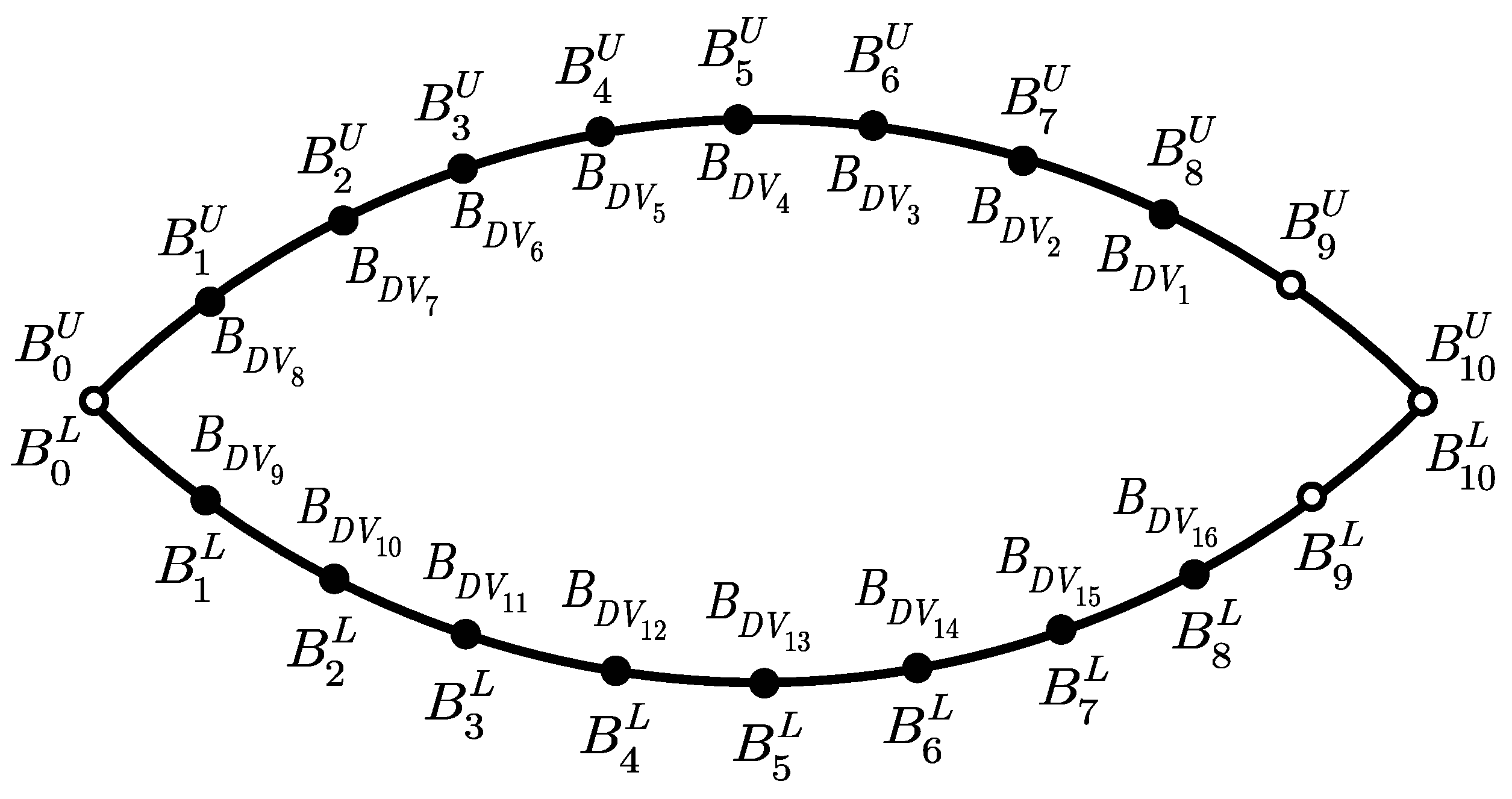
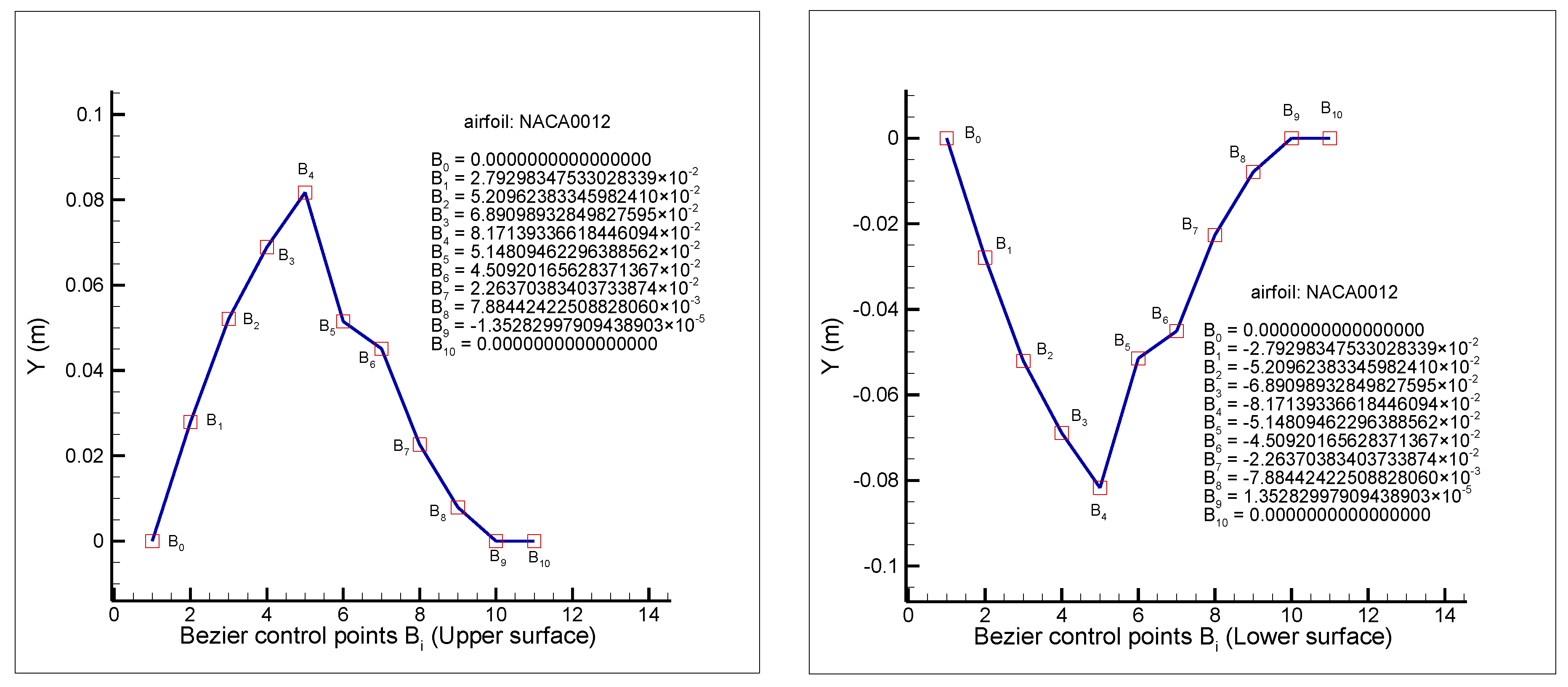
Here, in the aerodynamic shape optimization, the design variables were the Bezier control points (), as shown in Figure 3. The first and last two Bezier control points on the upper and the lower surfaces of the airfoil (hollow circles in Figure 3) were fixed and not considered to bedesign variables.For the ease of coding, the design variables were numbered consistent with the node numbering on the airfoil surface (see Appendix C). In other words, the design variables were numbered from right to left on the upper surface and from left to right on the lower surface (see Figure 3). The reason for fixing two control points adjacent to the airfoil trailing edge ( and ) was that the values of these two control points were very small ( and for the NACA0012 airfoil, as shown in Figure 4), especially given that they should be multiplied by another small variable (finite-difference step-size: see Equation (17)), and even the double-precision calculations of the flow solver (here ANSYS Fluent) may not be able to detect the change of the pressure of the perturbed nodes. Thus, the computation of the sensitivity coefficients using the finitedifference method for these two control points would be problematic and would result in a zero sensitivity coefficient due to the subtraction of nearly equal terms. The complex-step derivative approximation is a remedy for this issue if one has access to the solver source code to substitute all real type variable declarations with complex declarations and define all functions and operators that are not defined for complex arguments [22]. However, in this study, the two control points mentioned above were fixed and are not considered as design variables.
3.2. Objective Function
The aerodynamic shape optimization problem of interest here consistedof the minimization of the drag () to lift () ratio, , at a fixedangle of attack . This was an unconstrained optimization problem since no constraint was considered for it.
The objective function for this case is:
where
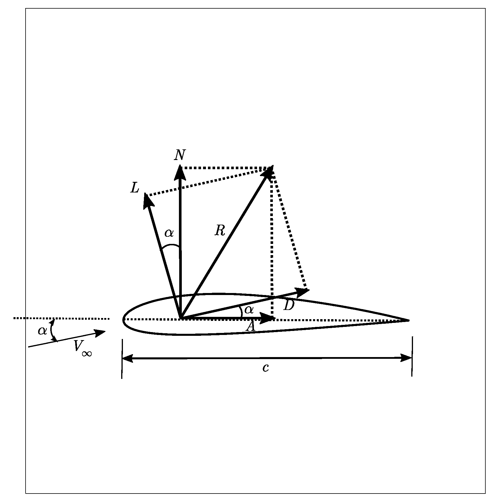
and and are axial and normal forces, respectively (Figure 5) [23]. We can write the drag and lift forces as follows:
Therefore, the objective function becomes:
3.3. Sensitivity Analysis
The sensitivity analysis in gradient-based optimization is concerned with the computation of the derivative of the objective function with respect to the unknown variables. Suppose we wish to calculate the sensitivity of the objective function defined by Equation (10) to the Bezier control points (). This can be mathematically expressed as:
The derivatives on the right-hand side of Equation (11) can be evaluated by taking the derivative of drag , Equation (8), and lift , Equation (9) with respect to the design variables , as follows:
Factoring , we obtain:
In a similar fashion, we obtain:
Factoring , we obtain:
Thus, the derivative of the objective function, Equation (10) becomes:
The sensitivity coefficients may be computed using the finitedifference method, which is chosen for the simplicity of implementation. Suppose we wish to calculate the sensitivity of the pressure of nodes on the airfoil surface, , to the -coordinate of the 16 Bezier control points ( (), 8 for each of the upper and lower surfaces)in this study. The sensitivity analysis can be performed by introducing a small perturbation to the -coordinate of each of the Bezier control points. The grid generation (using perturbed values for the Bezier control points) and flow problem may be solved to obtain the new values for the pressure . Using these values for the pressure, the dependency of the pressure on the perturbation of the -position of Bezier control points can be evaluated. The central finitedifference method is used to compute these sensitivities as follows:
In this study, the finitedifference step-size was . The term is the perturbation in the -position of the Bezier control point . Since the sensitivity of each pressure to each -position of the Bezier control point () is required, the computation of the sensitivity coefficients using this method requires 2 × (total number of control points − total number of fixed control points) = 2 × [2(11) − 2(3)] = 32 additional solutions of the flow problem at each iteration.
Moreover, the terms can be calculated using Equation (4). By having the value of the pressure at each node from the solution of flow equations (here, the Euler equations are used), the drag and the lift can be calculated using Equations (8) and (9), respectively. The angle of attack is given a priori and is constant. The airfoil surface coordinates, and , are also known from the Bezier curve equation (here, the are constant and do not change in the optimization process).
4. Optimization Method
In this study, the unconstrained nonlinear minimization problem was solved using Broyden-Fletcher-Goldfarb-Shanno (BFGS) method (a quasi-Newton method). The quasi-Newton method is a gradient-based optimization method thatuses an approximation of the Hessian matrix or the inverse of a Hessian matrix [24]. In the BFGS method, an approximate inverse of the Hessian matrix, , is updated iteratively until an optimal solution is found. The steps of the aerodynamic shape optimization using the BFGS method as implemented in this study are as follows.
- (1)
- Specify the physical domain; the boundary conditions; the problem conditions, such as the free stream Mach number; and the angle of attack.
- (2)
- Generate structured or unstructured grids over the domain. The airfoil surface is generated using aBezier curve of degree .
- (3)
- Solve the flow problem regarding finding the pressure values at thegrid points of the physical domain and hence the airfoil surface.
- (4)
- Using Equations (8) and (9), compute the objective function Equation (10).
- (5)
- Compute the sensitivity coefficients using Equation (17).
- (6)
- Compute the gradient direction using Equation (16).
- (7)
- The initial approximate inverse of Hessian matrix, , is taken as the identity matrix, namely .
- (8)
- Compute the direction of descent using the following equation:
- (9)
- Compute the search step length . An explicit expression for computing the search step length will be presented later.
- (10)
- Evaluate the new values of the design variables (Bezier curve control points) using the following equation:
- (11)
- Set the next iteration and return to step 2. Update the approximate inverse of the Hessian matrix as [24]:where:
There exists no exact search step length for highly nonlinear aerodynamic shape optimization problems. Therefore, an inexact step length using line search methods, such as backtracking, is determined and it is chosen in such a way that some conditions, such as Wolfe conditions, are satisfied [13,21,25]. Here, we present a novel method to obtain an exact step length in aerodynamic shape optimization problems involving the unconstrained minimization of common objective function definitions, such as drag and the drag-to lift-ratio. The formulation given here is concerned with the Bezier curve only but it can be extended to other airfoil parameterization methods.
Exact Step Length
The exact step length can be obtained as:
For simplicity, let and (), and suppose, for generality, that the Bezier control points associated with the trailing and leading edges are considered fixed (they are not considered as design variables). Thus, we can write:
where is divided into () for the upper surface and () for the lower surface. To obtain the exact step length , we minimize with respect to as follows:
Since , the indices in Equation (26) do not include . Equation (26) is the same as Equation (8) with the rearrangement of terms being with respect to rather than . From the definition of the Bezier curve, Equations (1) and (2)), we can write the drag, Equation (26) as:
Using (Equation (24)), we can write:
Afterexpanding, we obtain:
Using the identity , we can write the above expression as:
Therefore, we obtain
which is the exact step length. As can be seen from Equation (31), the value of the exact step length depends on the gradient of the objective function and it is independent of the method used for calculating the gradient. In other words, one can calculate the gradient with any available method, such as the adjoint method, the finitedifference method, etc., and then use Equation (31) to calculate the exact step length. It can be concluded that an inaccuracy in computing the gradient of the objective function or the approximate inverse of Hessian matrix can give rise to an inaccuracy in calculating the exact step length.
For the sake of simplicity, the derivation of the above general step length expression is presented for the Bezier curve of degree 10 and is given in Appendix A and a Fortran code to calculate it is given in Appendix D. The derivation of the exact step length for other forms of the objective function, such as drag minimization and lift-constrained drag minimization, is given in Appendix B.
5. Results
As mentioned previously, the objective of the aerodynamic shape optimization problem considered in this study was to minimize the drag-to-lift ratio (which is equivalent to the maximization of the lift-to-drag ratio) for an airfoil moving in a steady inviscid transonic flow through the implementation of the exact step length in a gradient-based optimization algorithm. The following test case is presented to investigate the accuracy and performance of the derived step length.
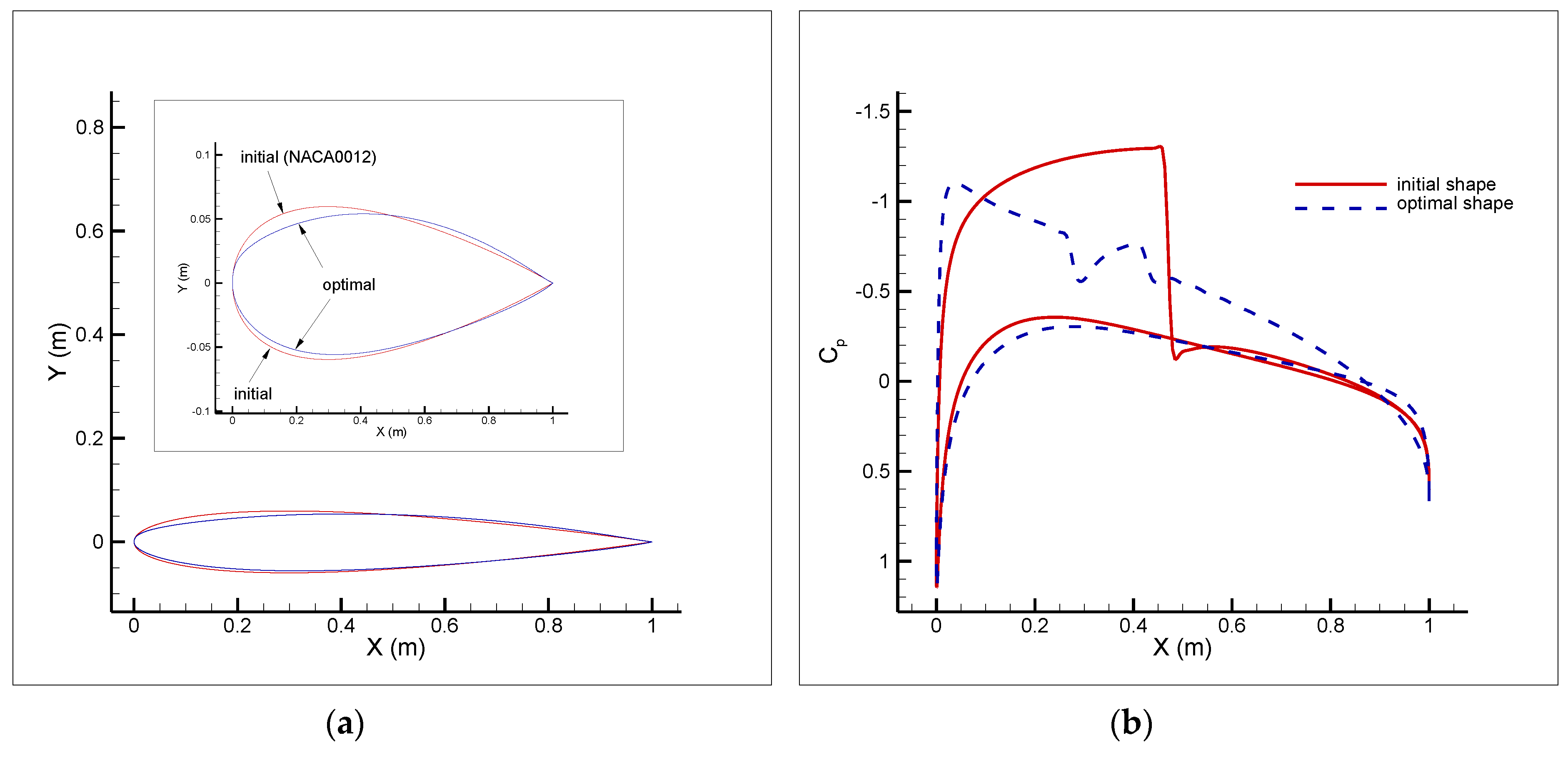
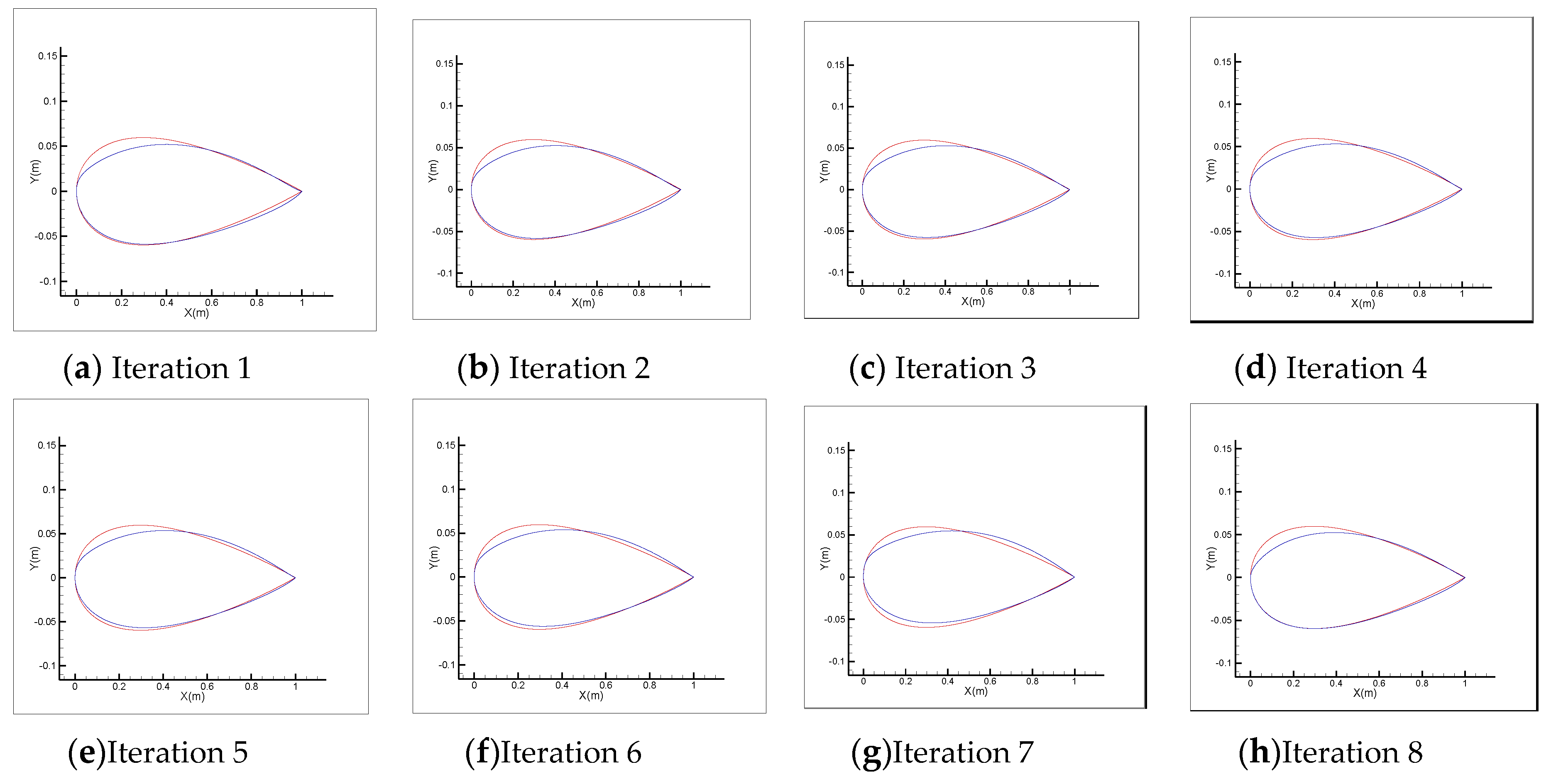
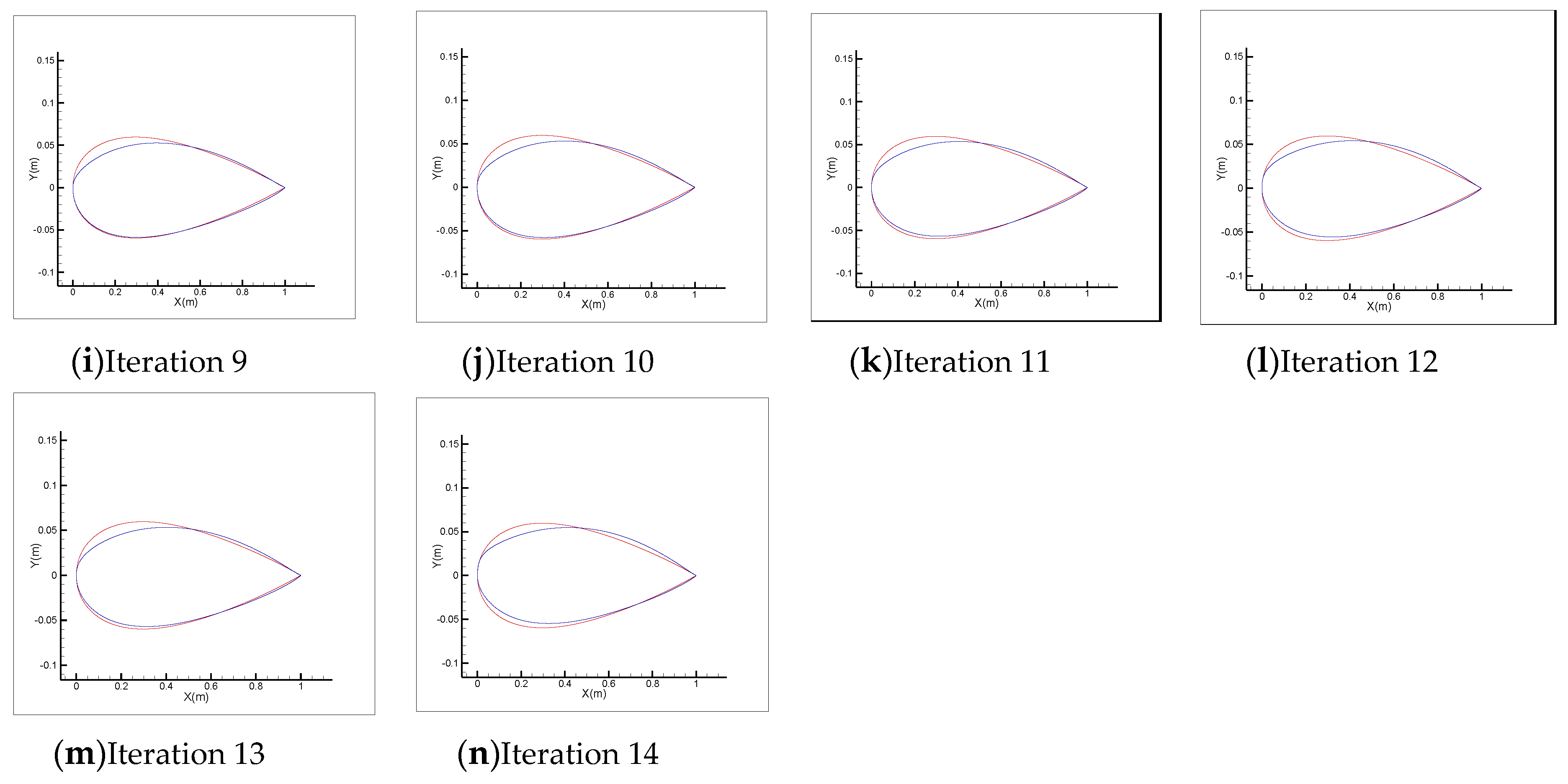
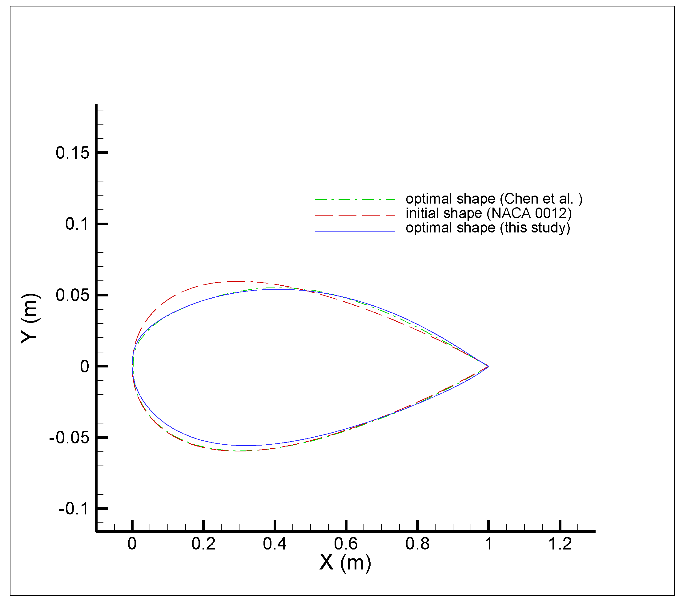
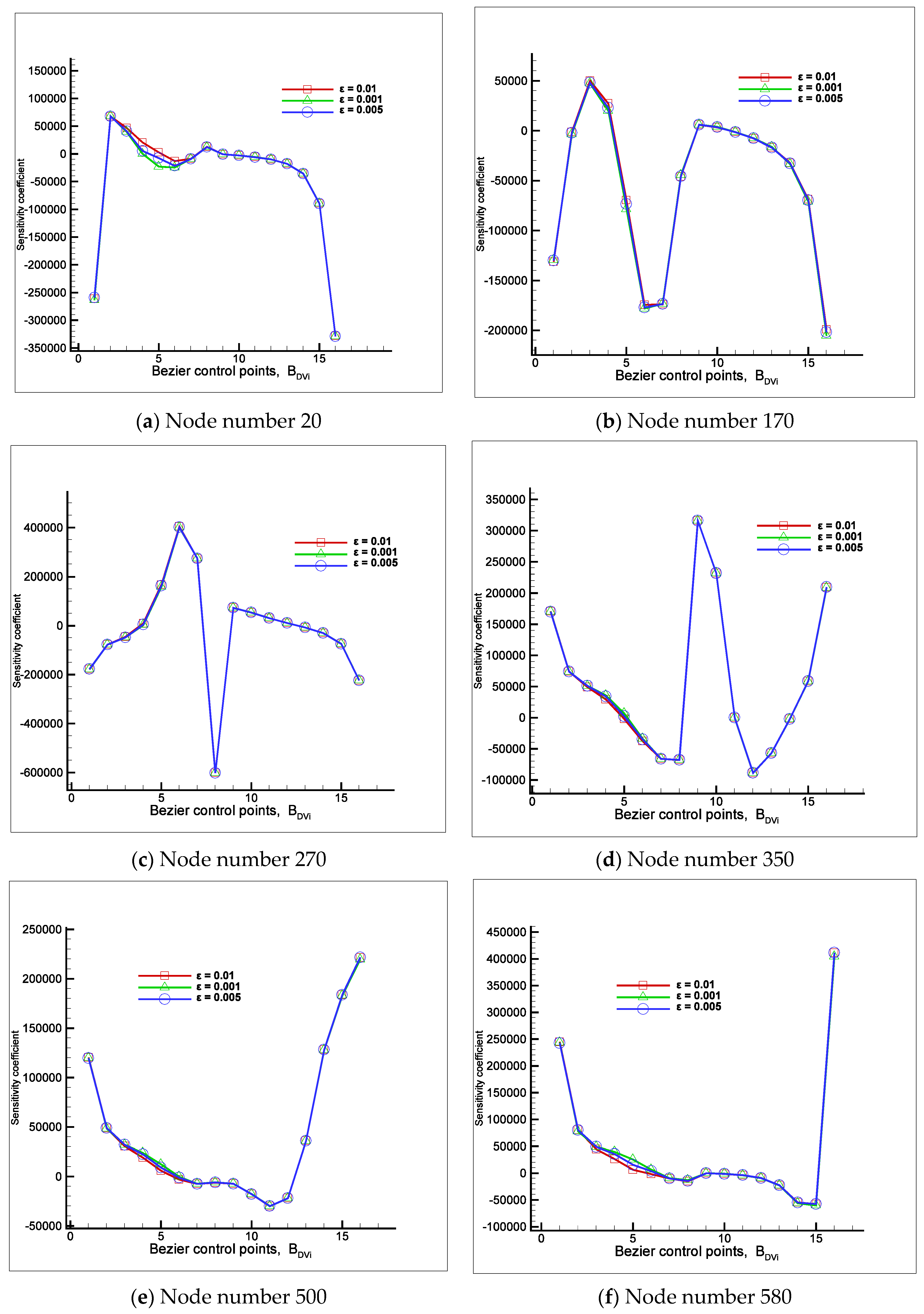
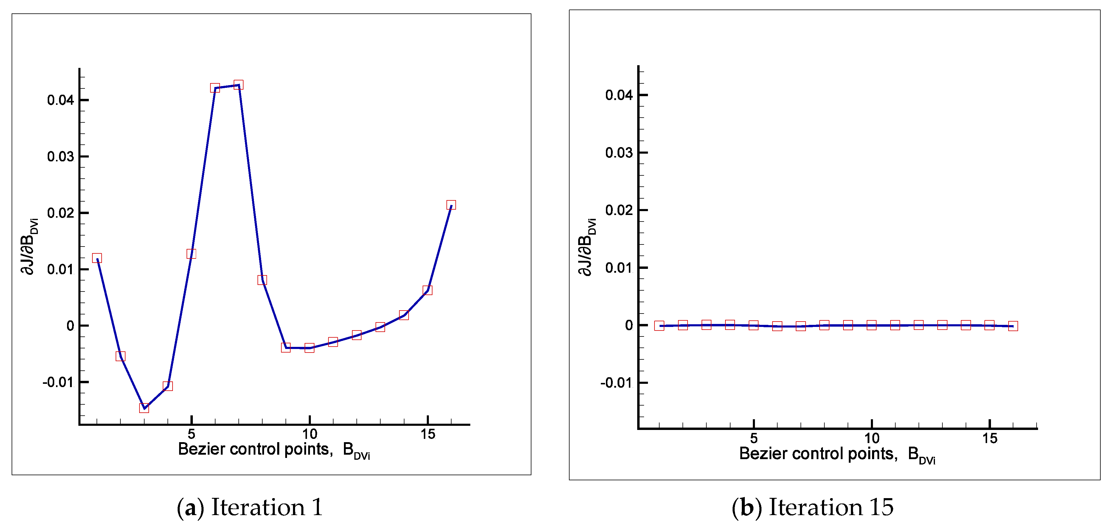
Test Case: A NACA 0012 airfoil operating at a fixed angle of attack of and a free-stream Mach number of 0.75 was considered for this test case as theinitial shape and flow conditions. The free stream pressure was . There was a strong shock at half of the airfoil chord length on the upper surface. Since there was shock-induced pressure drag on the airfoil inthese operating conditions, we aimedto optimize the airfoil to eliminate or weaken the shock as much as possible. The initial drag and lift forces were and , respectively (this means that for the initial airfoil, NACA 0012, inthese flow conditions,). The initial drag and lift coefficients were and , respectively, which are in excellent agreement with and in Carpentieri et al. [26]. As shown in Table 1, the drag and lift forces of the optimal shape were and , respectively (this means that for the optimal airfoil,, which was an approximately 11.6 times increase in the value of (). A substantial decrease in the drag (from to ) using only 16 design variables was achieved. Moreover, the drag and lift coefficients of the optimal shape were and , respectively. A structured O-grid (see Figure 6) with nodes on the airfoil surface and 109 nodes in the normal direction to the airfoil surface was generated. The inviscid transonic flow equations (Euler equations) were solved using the ANSYS Fluent software to compute the pressure at each node on the airfoil surface (for unperturbed and perturbed shapes foreach iteration). The computed pressures were then substituted into Equation (17) to calculate the sensitivity coefficients needed to compute the gradient of the objective function. A comparison of the initial shape (NACA 0012 airfoil) and the optimal one, as well as the corresponding surface pressure coefficients, is shown in Figure 7a,b, respectively. As can be seen, the shock on the initial shape was eliminated in the optimal shape. The static pressure distributions of the initial and optimal shapes are depicted in Figure 8a,b, respectively. A comparison of the initial and updated shape at each iteration is shown in Figure 9. As can be seen in Figure 9, the shock waseliminated or significantly weakened at each iteration (it is apparent from the value of the drag force given in Table 1, as well as from the thinner leading edge in the updated airfoils). The optimal shape is also in good agreement with the optimal shape in References [26,27]. A comparison of the initial shape (NACA 0012) and the optimal shapes obtained in Chen et al. [27] and from our study is shown in Figure 10. As can be seen, the upper surface shapes in both optimal shapes wereshock-free, which resulted in the minimum drag in both shapes (as can be seen in Table 1, the majority of the reduction in the objective function in the test case was due to the decrease in the drag value). The history of the objective function is shown in Figure 11. The value of the objective function was substantially reduced by 99.4% and most of the reduction was obtained in the first iteration. The optimization process was continued for 15 iterations. The value of the exact step length used in the BFGS optimization method (using Equation (31) or Equation (A5)) is plotted in Figure 12. At iteration 6, the negative value for the step length was obtained (). The minimum value for the objective function was obtained at iteration 6; however, as this value was obtained by a negative step length, the optimization process was continued further. The sensitivity coefficients at some arbitrary nodal points (node numbers 20, 170, and 270 on the upper surface and node numbers 350, 500, and 580 on the lower surface; there are nodes on each surface of the airfoil) on the airfoil surface using three different finite-difference step-sizes , , and are depicted in Figure 13. As shown, the sensitivity coefficients at each node using the three step-sizes were in good agreement. However, in this study, the finite-difference step-size was used to calculate the sensitivity coefficients using Equation (17). The gradients of the objective function with respect to the design variables () for the first and last iterations(iterations 1 and 15) are shown in Figure 14a,b, respectively, representing a significant decrease in the norm of the gradient (from to ; a reduction) to infer the optimal shape.
It should be emphasized that the gradient of the objective function with respect to the design variables was computed using the finitedifference method. More accurate results are expected if the gradient computation is accomplished with more accurate methods, such as the adjoint method or the complex-step method.
6. Conclusions
This study aimed to develop a novel and exact step length for gradient-based aerodynamic shape optimization problems. The steady inviscid transonic flow governed by the Euler equations was considered and the Euler equations were solved usingthe finite element solver ANSYS Fluent. Minimization of the drag-to-lift ratio (which is equivalent to the maximization of the lift-to-drag ratio) was performed. The quasi-Newton (BFGS) method was employed to minimize the defined objective function. The airfoil (NACA 0012) surface was parameterized usinga Bezier curve and an explicit exact step length was derived for the unconstrained minimization problem. We showed that the value of the exact step length dependedon both the values of the gradient of the objective function and the Bezier control points. A test case was presented to investigate the effect of the exact step length on the shape optimization process. Using the exact step length, the optimal shape was obtained within a few iterations with a substantial reduction in the objective function value.
Author Contributions
Conceptualization, F.M. and B.E.; Data curation, F.M.; Formal analysis, F.M.; Funding acquisition, F.M. and B.E.; Investigation, F.M.; Methodology, F.M. and B.E.; Resources, F.M. Software, F.M.; Supervision, B.E.; Validation, F.M.; Visualization, F.M.; Writing—original draft, F.M.; Writing—review & editing, F.M. and B.E. All authors have read and agreed to the published version of the manuscript.
Funding
This research was supported by funding from the European Union’s Horizon 2020 research and innovation program under the Marie Skłodowska-Curie grant agreement no. 663830.
Conflicts of Interest
The authors declare no conflict of interest.
Nomenclature
| Bezier curve control point | |
| direction of descent at iteration | |
| objective function | |
| Bernstein basis polynomial | |
| degree of the Bernstein basis polynomial in Bezier curve | |
| pressure | |
| and/or in the Bezier curve expression | |
| parameter used in the Bezier curve, | |
| Cartesian coordinates in the physical domain | |
| search step length at iteration | |
| design variable | |
| iteration number |
Appendix A
Using , we can write Equation (A1) as:
After factoring, we obtain:
which will be:
Thus, the exact step length is obtained as being:
The Fortran 77 code used for calculation of the exact step length given by Equation (A5) is presented in Appendix D.
Appendix B
Appendix B.1. Other Forms of the Objective Function
Appendix B.1.1. Drag Minimization
It is worth mentioning at this stage that the above expression for the step length is equally valid for drag minimization problems as well. In such a case, we can express the objective function as:
Thus, we can write
where the term can be computed usingEquation (13). In a similar fashion to Equation (25), to derive an exact expression for the step length, we can write:
which results in the same expression for the step length given in Equation (31) (or Equation (A5)).
Appendix B.1.2. Lift-Constrained Drag Minimization
In such a case, we can express the objective function as:
The equality constraint, , can be explicitly incorporated into the objective function, , toconvert the constrained optimization problem to an equivalent unconstrained one. If
Then, from Equation (7), we have:
Therefore, we can write:
By substituting into the drag force expression (Equation (6)), we have:
Using , the drag force expression simplifies to:
or
Now the objective function expression to be minimized is:
The gradient expression is:
After simplifying (because the lift force is constant, , we have ), we obtain:
Equation (A17) is the gradient expression for the equivalent unconstrained optimization form of the lift-constrained drag minimization problem.
To obtain an exact step length for this case, it is necessary to have . From Equation (A16), after a rearrangement of terms with respect to rather than , we can write:
In a similar procedure to the previous cases, we can obtain the exact step length as being:
or for the Bezier curve of degree 10 used in this study as being:
Note that in this equation, there is no . term as the initial lift force, which should be constant during the optimization process.
Appendix C
The Fortran code for converting the Bezier control points to the design variables is as follows:
- C n is the degree of Bezier curve
- C CPN is the Control Points Number (which is n+1=10+1=11 here)
- C B_Y_T and B_Y_B is Bezier control points associated with the top and
- C bottom surfaces, respectively
- C B_Y is the Bezier design variable (see Figure 3: Two Bezier control
- C points adjacent to trailing edge are not considered as design C
- C variables in this code;therefore, there are eight design variables on top and
- C surface and eight design variables on the bottom surface)
- n=10
- CPN=n+1
- DO I=1,CPN-3
- B_Y(I,1)=B_Y_T(CPN-I-1,1)
- ENDDO
- DO I=CPN-3+1,2*CPN-6
- B_Y(I,1)=B_Y_B(I-CPN+3+1,1)
- ENDDO
Appendix D
- C STS stands for step-size (length) calculation
- C t_STS is associated with each node on the airfoil surface,
- C as defined in Figure 1
- C t_T is t for the top surface; t_B is t for the bottom surface
- C N is the number of nodes on airfoil surface
- DELTA1_TT=(1.0−0.0)/((N+1)/2−1)
- DELTA1_TB=(1.0−0.0)/((N+1)/2−1)
- t_T(1,1)=0.0
- t_T((N+1)/2,1)=1.0
- t_B(1,1)=0.0
- t_B((N+1)/2,1)=1.0
- DO I=2,(N+1)/2−1
- t_T(I,1)=t_T(I-1,1)+DELTA1_TT
- ENDDO
- DO I=2,(N+1)/2−1
- t_B(I,1)=t_B(I−1,1)+DELTA1_TB
- ENDDO
- t_STS(1,1)=1.0
- t_STS(1,(N+1)/2)=0.0
- t_STS(1,N)=1.0
- DO J=2,(N+1)/2−1
- t_STS(1,J)=t_T((N+1)/2+1−J,1)
- ENDDO
- DO J=(N+1)/2+1,N−1
- t_STS(1,J)=t_B(J−(N+1)/2+1,1)
- ENDDO
- C for the upper surface
- A(1)=0.0
- DO J=2,(N+1)/2−1
- A(1)=A(1)+10.0*(t_STS(1,J)**9)*((1.0−t_STS(1,J))**1)*
- +(PRESSURE(1,J)−PRESSURE(1,J−1))
- ENDDO
- A(2)=0.0
- DO J=2,(N+1)/2−1
- A(2)=A(2)+45.0*(t_STS(1,J)**8)*((1.0-t_STS(1,J))**2)*
- +(PRESSURE(1,J)−PRESSURE(1,J−1))
- ENDDO
- A(3)=0.0
- DO J=2,(N+1)/2−1
- A(3)=A(3)+120.0*(t_STS(1,J)**7)*((1.0−t_STS(1,J))**3)*
- +(PRESSURE(1,J)−PRESSURE(1,J−1))
- ENDDO
- A(4)=0.0
- DO J=2,(N+1)/2−1
- A(4)=A(4)+210.0*(t_STS(1,J)**6)*((1.0−t_STS(1,J))**4)*
- +(PRESSURE(1,J)−PRESSURE(1,J−1))
- ENDDO
- A(5)=0.0
- DO J=2,(N+1)/2−1
- A(5)=A(5)+252.0*(t_STS(1,J)**5)*((1.0−t_STS(1,J))**5)*
- +(PRESSURE(1,J)−PRESSURE(1,J−1))
- ENDDO
- A(6)=0.0
- DO J=2,(N+1)/2−1
- A(6)=A(6)+210.0*(t_STS(1,J)**4)*((1.0−t_STS(1,J))**6)*
- +(PRESSURE(1,J)−PRESSURE(1,J-1))
- ENDDO
- A(7)=0.0
- DO J=2,(N+1)/2−1
- A(7)=A(7)+120.0*(t_STS(1,J)**3)*((1.0−t_STS(1,J))**7)*
- +(PRESSURE(1,J)−PRESSURE(1,J−1))
- ENDDO
- A(8)=0.0
- DO J=2,(N+1)/2−1
- A(8)=A(8)+45.0*(t_STS(1,J)**2)*((1.0−t_STS(1,J))**8)*
- +(PRESSURE(1,J)−PRESSURE(1,J−1))
- ENDDO
- A(9)=0.0
- DO J=2,(N+1)/2−1
- A(9)=A(9)+10.0*(t_STS(1,J)**1)*((1.0−t_STS(1,J))**9)*
- +(PRESSURE(1,J)−PRESSURE(1,J−1))
- ENDDO
- C for the lower surface
- A(10)=0.0
- DO J=(N+1)/2+1,N−1
- A(10)=A(10)+10.0*(t_STS(1,J)**1)*((1.0−t_STS(1,J))**9)*
- +(PRESSURE(1,J)−PRESSURE(1,J−1))
- ENDDO
- A(11)=0.0
- DO J=(N+1)/2+1,N−1
- A(11)=A(11)+45.0*(t_STS(1,J)**2)*((1.0−t_STS(1,J))**8)*
- +(PRESSURE(1,J)−PRESSURE(1,J−1))
- ENDDO
- A(12)=0.0
- DO J=(N+1)/2+1,N−1
- A(12)=A(12)+120.0*(t_STS(1,J)**3)*((1.0−t_STS(1,J))**7)*
- +(PRESSURE(1,J)−PRESSURE(1,J−1))
- ENDDO
- A(13)=0.0
- DO J=(N+1)/2+1,N−1
- A(13)=A(13)+210.0*(t_STS(1,J)**4)*((1.0−t_STS(1,J))**6)*
- +(PRESSURE(1,J)−PRESSURE(1,J−1))
- ENDDO
- A(14)=0.0
- DO J=(N+1)/2+1,N−1
- A(14)=A(14)+252.0*(t_STS(1,J)**5)*((1.0−t_STS(1,J))**5)*
- +(PRESSURE(1,J)−PRESSURE(1,J−1))
- ENDDO
- A(15)=0.0
- DO J=(N+1)/2+1,N−1
- A(15)=A(15)+210.0*(t_STS(1,J)**6)*((1.0−t_STS(1,J))**4)*
- +(PRESSURE(1,J)−PRESSURE(1,J-1))
- ENDDO
- A(16)=0.0
- DO J=(N+1)/2+1,N−1
- A(16)=A(16)+120.0*(t_STS(1,J)**7)*((1.0−t_STS(1,J))**3)*
- +(PRESSURE(1,J)−PRESSURE(1,J−1))
- ENDDO
- A(17)=0.0
- DO J=(N+1)/2+1,N−1
- A(17)=A(17)+45.0*(t_STS(1,J)**8)*((1.0−t_STS(1,J))**2)*
- +(PRESSURE(1,J)−PRESSURE(1,J−1))
- ENDDO
- A(18)=0.0
- DO J=(N+1)/2+1,N−1
- A(18)=A(18)+10.0*(t_STS(1,J)**9)*((1.0−t_STS(1,J))**1)*
- +(PRESSURE(1,J)−PRESSURE(1,J−1))
- ENDDO
- C terms in Equation (24):
- DO I=1,2*CPN−4
- b_STS(I,1)=0.0
- DO L=1,2*CPN−4
- b_STS(I,1)=b_STS(I,1)+BY_BFGS(I,L)*DELTA_SY(L,1)
- ENDDO
- ENDDO
- DO I=1,2*CPN−4
- a_STS(I,1)=B_Y(I,1)
- ENDDO
- C calculation of beta (exact step-size):
- C terms in numerator of Equation (A5)
- BETA1_KY=0.0
- DO I=1,2*CPN−4
- BETA1_KY=BETA1_KY+a_STS(I,1)*A(I)
- ENDDO
- C terms in the denominator of Equation (A5)
- BETA2_KY=0.0
- DO I=1,2*CPN−4
- BETA2_KY=BETA2_KY+b_STS(I,1)*A(I)
- ENDDO
- C Equation (A5):
- BETA_KY=(COS(PI*AOA/180.0)*BETA1_KY+NORMAL_FORCE*
- +SIN(PI*AOA/180.0))/(COS(PI*AOA/180.0)*BETA2_KY)
References
- Hicks, R.M.; Murman, E.M.; Vanderplaats, G.N. An Assessment of Airfoil Design by Numerical Optimization; National Technical Information Service: Springfield, VA, USA, 1974. [Google Scholar]
- Hicks, R.M.; Henne, P.A. Wing design by numerical optimization. J. Aircr. 1978, 15, 407–412. [Google Scholar] [CrossRef]
- Pironneau, O. On optimum design in fluid mechanics. J. Fluid Mech. 1974, 64, 97–110. [Google Scholar] [CrossRef]
- Jameson, A. Aerodynamic design via control theory. J. Sci. Comput. 1988, 3, 233–260. [Google Scholar] [CrossRef] [Green Version]
- Jameson, A. Optimum aerodynamic design using CFD and control theory. In Proceedings of the 12th Computational Fluid Dynamics Conference, San Diego, CA, USA, 19–22 June 1995; p. 1729. [Google Scholar]
- Jameson, A. Automatic design of transonic airfoils to reduce the shock induced pressure drag. In Proceedings of the 31st Israel Annual Conference on Aviation and Aeronautics, Tel Aviv, Israel, 21–22 February 1990; pp. 5–17. [Google Scholar]
- Jameson, A.; Reuther, J. Control theory based airfoil design using the Euler equations. In Proceedings of the 5th Symposium on Multidisciplinary Analysis and Optimization, Panama City Beach, FL, USA, 7–9 September 1994; p. 4272. [Google Scholar]
- Lyu, Z.; Kenway, G.K.; Martins, J.R. Aerodynamic shape optimization investigations of the common research model wing benchmark. AIAA J. 2014, 53, 968–985. [Google Scholar] [CrossRef] [Green Version]
- Papadimitriou, D.I.; Papadimitriou, C. Aerodynamic shape optimization for minimum robust drag and lift reliability constraint. Aerosp. Sci. Technol. 2016, 55, 24–33. [Google Scholar] [CrossRef]
- Srinath, D.N.; Mittal, S. An adjoint method for shape optimization in unsteady viscous flows. J. Comput. Phys. 2010, 229, 1994–2008. [Google Scholar] [CrossRef]
- Economon, T.D.; Palacios, F.; Copeland, S.R.; Lukaczyk, T.W.; Alonso, J.J. SU2: An open-source suite for multiphysics simulation and design. AIAA J. 2015, 54, 828–846. [Google Scholar] [CrossRef]
- He, X.; Li, J.; Mader, C.A.; Yildirim, A.; Martins, J.R. Robust aerodynamic shape optimization—From a circle to an airfoil. Aerosp. Sci. Technol. 2019, 87, 48–61. [Google Scholar] [CrossRef]
- Mohammadi, B.; Pironneau, O. Applied Shape Optimization for Fluids; Oxford University Press: Oxford, UK, 2009. [Google Scholar]
- Thevenin, D.; Janiga, G. Optimization and Computational Fluid Dynamics; Springer Science & Business Media: Berlin, Germany, 2008. [Google Scholar]
- Skinner, S.N.; Zare-Behtash, H. State-of-the-art in aerodynamic shape optimisation methods. Appl. Soft Comput. 2018, 62, 933–962. [Google Scholar] [CrossRef]
- Giles, M.B.; Pierce, N.A. An introduction to the adjoint approach to design. Flow Turbul. Combust. 2000, 65, 393–415. [Google Scholar] [CrossRef]
- Giles, M.B.; Duta, M.C.; M-uacute, J.D.; Pierce, N.A. Algorithm developments for discrete adjoint methods. AIAA J. 2003, 41, 198–205. [Google Scholar] [CrossRef] [Green Version]
- Elliott, J.; Peraire, J. Aerodynamic design using unstructured meshes. In Proceedings of the Fluid Dynamics Conference, New Orleans, LA, USA, 17–20 June 1996; p. 1941. [Google Scholar]
- Nemec, M.; Zingg, D.W. Newton-Krylov algorithm for aerodynamic design using the Navier-Stokes equations. AIAA J. 2002, 40, 1146–1154. [Google Scholar] [CrossRef] [Green Version]
- Anderson, W.K.; Venkatakrishnan, V. Aerodynamic design optimization on unstructured grids with a continuous adjoint formulation. Comput. Fluids 1999, 28, 443–480. [Google Scholar] [CrossRef] [Green Version]
- Nocedal, J.; Wright, S. Numerical Optimization; Springer: New York, NY, USA, 2006. [Google Scholar]
- Martins, J.R.; Sturdza, P.; Alonso, J.J. The complex-step derivative approximation. ACM Trans. Math. Softw. 2003, 29, 245–262. [Google Scholar] [CrossRef] [Green Version]
- Anderson, J.D. Fundamentals of Aerodynamics; McGraw-Hill Education: New York, NY, USA, 2016. [Google Scholar]
- Rao, S.S. Engineering Optimization: Theory and Practice; Wiley: Hoboken, NJ, USA, 2009. [Google Scholar]
- Butenko, S.; Pardalos, P.M. Numerical Methods and Optimization: An Introduction; Taylor & Francis: Abingdon-on-Thames, UK, 2014. [Google Scholar]
- Carpentieri, G.; Koren, B.; van Tooren, M.J.L. Adjoint-based aerodynamic shape optimization on unstructured meshes. J. Comput. Phys. 2007, 224, 267–287. [Google Scholar] [CrossRef] [Green Version]
- Chen, W.; Zhang, W.; Liu, Y.; Kou, J. Accelerating the convergence of steady adjoint equations by dynamic mode decomposition. Struct. Multidiscip. Optim. 2020. [Google Scholar] [CrossRef]
Figure 1.
The node definition on the airfoil surface.

Figure 2.
Definition of the parameter used in the Bezier curve.

Figure 3.
Definition of the design variables used for aerodynamic shape optimization. Here, the coordinates of the Bezier control points were not real and were plotted this way for the sake of simplicity in the definition.
Figure 3.
Definition of the design variables used for aerodynamic shape optimization. Here, the coordinates of the Bezier control points were not real and were plotted this way for the sake of simplicity in the definition.

Figure 4.
The values of the Bezier control points for the upper and lower surfaces of a NACA 0012 airfoil.
Figure 4.
The values of the Bezier control points for the upper and lower surfaces of a NACA 0012 airfoil.

Figure 5.
Resultant aerodynamic force and the components into which it splits [23].
Figure 5.
Resultant aerodynamic force and the components into which it splits [23].

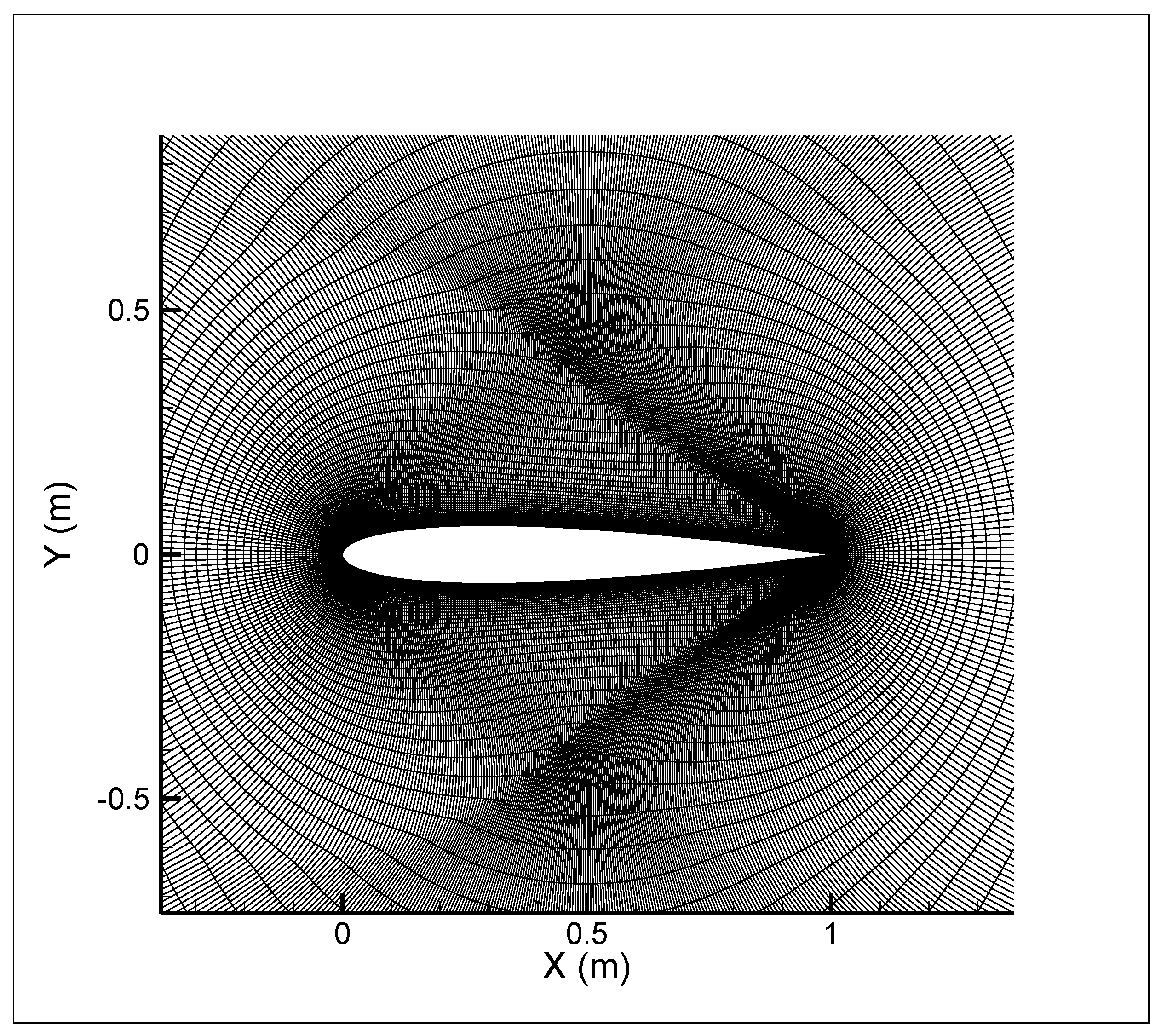
Figure 6.
Structured mesh (hyperbolic O-grid) used for solving the transonic flow equations. The size of the mesh was .
Figure 6.
Structured mesh (hyperbolic O-grid) used for solving the transonic flow equations. The size of the mesh was .

Figure 7.
Comparison of initial and optimal airfoils used in the transonic flow shape optimization (a) and the corresponding airfoil surface pressure coefficients (b).
Figure 7.
Comparison of initial and optimal airfoils used in the transonic flow shape optimization (a) and the corresponding airfoil surface pressure coefficients (b).

Figure 8.
Static pressure distribution for the initial shape (NACA 0012) (a) and the optimal shape (at iteration 15) (b).
Figure 8.
Static pressure distribution for the initial shape (NACA 0012) (a) and the optimal shape (at iteration 15) (b).

Figure 9.
Comparison of the initial shape (NACA 0012) and the updated shape at (a–n) iteration 1 to iteration 14.
Figure 9.
Comparison of the initial shape (NACA 0012) and the updated shape at (a–n) iteration 1 to iteration 14.


Figure 10.
Comparison of the initial shape (NACA 0012), the optimal shape from our study, and the optimal shape from Chen et al. [27]; it shows a good agreement between the optimal shapes and an excellent agreement between the optimal upper surfaces where the shock was eliminated.
Figure 10.
Comparison of the initial shape (NACA 0012), the optimal shape from our study, and the optimal shape from Chen et al. [27]; it shows a good agreement between the optimal shapes and an excellent agreement between the optimal upper surfaces where the shock was eliminated.

Figure 11.
History of the objective function, , during the shape optimization process.

Figure 12.
Exact step length value during the shape optimization process.

Figure 13.
Sensitivity coefficients at some arbitrary nodes using three different finite-difference stepsizes.
Figure 13.
Sensitivity coefficients at some arbitrary nodes using three different finite-difference stepsizes.

Figure 14.
The gradient of the objective function with respect to the design variables at iteration 1 (a) and iteration 15 (b).
Figure 14.
The gradient of the objective function with respect to the design variables at iteration 1 (a) and iteration 15 (b).


Table 1.
Results for the test case.
| 0 (initial shape) | 9.10775 × 10⁻⁴ | - | 515.760 | 17,090.000 | 1.294 × 10⁻² | 0.42867 |
| 1 | 1.97841 × 10⁻⁵ | 0.5534 | 34.032 | 7651.200 | 8.536 × 10⁻⁴ | 0.19191 |
| 2 | 1.34569 × 10⁻⁵ | 1.6872 | 35.644 | 9716.600 | 8.940 × 10⁻⁴ | 0.24372 |
| 3 | 1.06817 × 10⁻⁵ | 1.1510 | 38.239 | 11,700.000 | 9.591 × 10⁻⁴ | 0.29348 |
| 4 | 9.92128 × 10⁻⁶ | 2.4779 | 40.664 | 12,910.000 | 1.020 × 10⁻³ | 0.32381 |
| 5 | 8.40409 × 10⁻⁶ | 0.0188 | 40.980 | 14,136.000 | 1.028 × 10⁻³ | 0.35456 |
| 6 | 4.89131 × 10⁻⁶ | −1.2468 | 35.521 | 16,061.000 | 8.910 × 10⁻⁴ | 0.40284 |
| 7 | 1.50193 × 10⁻⁵ | 47.6144 | 72.886 | 18,807.000 | 1.828 × 10⁻³ | 0.47174 |
| 8 | 2.14748 × 10⁻⁵ | 2.8478 | 49.214 | 10,620.000 | 1.234 × 10⁻³ | 0.26638 |
| 9 | 1.66016 × 10⁻⁵ | 0.3450 | 48.401 | 11,879.000 | 1.214 × 10⁻³ | 0.29795 |
| 10 | 1.24568 × 10⁻⁵ | 0.2160 | 45.653 | 12,935.000 | 1.145 × 10⁻³ | 0.32445 |
| 11 | 7.33858 × 10⁻⁶ | 0.2599 | 38.305 | 14,140.000 | 9.608 × 10⁻⁴ | 0.35466 |
| 12 | 6.68139 × 10⁻⁶ | 0.0009 | 40.202 | 15,553.000 | 1.008 × 10⁻³ | 0.39011 |
| 13 | 8.65189 × 10⁻⁶ | 11.8508 | 40.162 | 13,654.000 | 1.007 × 10⁻³ | 0.34247 |
| 14 | 1.26244 × 10⁻⁵ | 1.8642 | 59.411 | 16,721.000 | 1.490 × 10⁻³ | 0.41941 |
| 15 | 5.73953 × 10⁻⁶ | 0.9977 | 36.142 | 15,086.000 | 9.065 × 10⁻⁴ | 0.37839 |
| - | 99.4% reduction | - | 93.0% reduction | 11.7% reduction | - | - |
© 2020 by the authors. Licensee MDPI, Basel, Switzerland. This article is an open access article distributed under the terms and conditions of the Creative Commons Attribution (CC BY) license (http://creativecommons.org/licenses/by/4.0/).
Share and Cite
MDPI and ACS Style
Mohebbi, F.; Evans, B. On an Exact Step Length in Gradient-Based Aerodynamic Shape Optimization. Fluids 2020, 5, 70. https://doi.org/10.3390/fluids5020070
AMA Style
Mohebbi F, Evans B. On an Exact Step Length in Gradient-Based Aerodynamic Shape Optimization. Fluids. 2020; 5(2):70. https://doi.org/10.3390/fluids5020070
Chicago/Turabian StyleMohebbi, Farzad, and Ben Evans. 2020. "On an Exact Step Length in Gradient-Based Aerodynamic Shape Optimization" Fluids 5, no. 2: 70. https://doi.org/10.3390/fluids5020070