Article

Optimisation of the Filament Winding Approach Using a Newly Developed In-House Uncertainty Model

1
The Advanced Sustainable Manufacturing Technologies (ASTUTE) Project, Faculty of Science and Engineering, Swansea University, Swansea SA1 8EN, UK
2
The Future Manufacturing Research Institute (FMRI), Faculty of Science and Engineering, Swansea University, Swansea SA1 8EN, UK
3
The Steel and Metals Institute (SaMI), Faculty of Science and Engineering, Swansea University, Swansea SA2 8PP, UK
*
Author to whom correspondence should be addressed.
Eng 2020, 1(2), 122-136; https://doi.org/10.3390/eng1020008
Submission received: 15 September 2020 / Revised: 6 October 2020 / Accepted: 10 October 2020 / Published: 13 October 2020

Abstract

:
The device under investigation in this paper consists of a float used to capture tidal energy, which is tethered by multiple flexible cables to a large barge-like reactor. The proposed float is made of a continuously wound glass-reinforced composite shell with stainless steel bolting plates integrated into the float walls to allow the connection of 5 stainless steel cables. Numerical computations are required to assess whether a delamination of the composite layers in the float is likely. The manufacturing of the device has various potential uncertainties that should be investigated, such as the number of the plies, the bond strength between the composite layers, and the fibre orientations of the composite material relative to the applied load. This paper provides a multi-level strategy to optimise the composite float system, which is manufactured from glass-reinforced plastic (GRP). In contrast to previous publications on the topic, the current work uses an efficient link between ANSYS Workbench and MATLAB through an in-house code that has been developed over 3 years. This allowed the whole process to be fully automated and to reduce the time and cost of the simulations. Previously, ANSYS APDL was linked to MATLAB, but limitations in terms of the geometry and boundary conditions made it impractical when compared to ANSYS Workbench for the simulation of complex features. This makes the current approach unique and rare when compared to the published work in the field. This approach allows the use of a huge number of trials and is able to reduce the number of parameters to be studied by selecting the most sensitive ones. Additionally, the developed tools may be used for the efficient, robust optimisation of the proposed structure. The current study has focused on exploring the effects of the fibre orientations and the optimum number of plies on the overall performance of the structure.

1. Introduction

1.1. Background

The device under investigation consists of a float that is tethered by multiple flexible cables to a large barge-like reactor to harvest tidal energy. The cables are attached to a hydraulic power take-off system that captures the energy from the relative movement between the float and the reactor, which is then converted to electricity. The proposed device has the potential to compete favourably with other available renewable technologies, since the proposed device relies on sea waves, which are more consistent than wind and offer an average power density of 2–3 W/m2, which is superior to that of wind (0.5 W/m2) and solar energy (0.1–0.3 W/m2) [1] Although several experiments have been conducted on the system, computational modelling of the device immersed in sea water is also required. The proposed float is made of a continuously wound glass-reinforced composite shell with stainless steel bolting plates integrated into the float walls to connect the float to a large barge on the seabed using 5 stainless steel cables, as shown in Figure 1. The barge hosts the energy harvesting devices that depend on the variation of the tension loads in the cables due to the constrained float movement. A sub-modelling technique is introduced with a layered (float) model and a solid (anchoring system) model to fully explore and assess the stress levels within each of the winding layers of the float. The integrity of the bonding between the cable connectors and the composite layers under normal operation will also be investigated, as it represents a major potential weakness in the integrity of the structure. In other words, the existence of high stress levels at the boundary between the anchoring system and the float under normal operation is one of the issues that might be encountered in the structure. In addition to locally altering the design in these zones to improve the structural response, it is necessary to perform further computations to assess if a delamination of the float layers is likely, taking into account the variable wave loading, i.e., the development of faults due to fatigue, which is beyond the scope of the current paper. The system suffers from various uncertainties, such as the number of plies in the top and bottom shells, the strength of the steel cable, the bond strength between the steel plates and the composite layers, the bond strength between the composite layers, and the fibre orientations of the composite material relative to the applied load. The current study will concentrate on exploring the effects of the fibre orientations and the number of plies on the overall performance of the structure.
The filament winding process consists of two main elements: a filament- or tape-type reinforcement and a matrix or resin. The process wraps a band of continuous resin-impregnated fibres around a rotating mandrel, which is then cured at room temperature or in an oven under prescribed pressure and temperature, as shown in Figure 2. The mechanical properties of the final product depend on the material, winding angle, fibre strength, resin chemistry, and curing cycles [2]. The filament winding process has become very popular due its the attractive properties, such as its high stiffness-to-weight ratios. Such properties have made this process widely used in many applications, such as in aerospace, hydrospace, and military applications. The reinforcement and the matrix can be tailor-made in order to satisfy particular properties. The winding pattern is controlled through the rotational speed of the mandrel and the movement of the fibre feed mechanism [3]. The mechanical properties of the filament-wound component are heavily influenced by the mechanical properties of the fibres, the surface interaction of the fibre and resin (interface), the amount of fibres in the composite, and the orientation of the fibres. The properties of the composite are highly direction-dependent and the fibres may be laid in the direction of the expected significant loading to ensure high integrity of the structure [3]. The helical winding process (see Figure 2) lays down the fibres at angles ranging from 5° to 85° relative to the longitudinal axis of the mandrel and lays the fibres in alternating positive and negative orientations [4].

1.2. The Winding Angle

The winding angle is defined as the angle between the laid-down fibres and the longitudinal axis of the cylindrical mandrel. Several studies have been conducted in order to find the approach that approximates and optimises the best combination of winding angles. Sulaiman et al. (2013) utilised a set of winding angle combinations ranging between 0° and 90°, i.e., [00°, 00°]s, [15°, −15°]s, [30°, −30°]s, [45°, −45°]s, [55°, −55°]s, [60°, −60°]s, [75°, −75°]s, and [90°, −90°]s orientations (where +ve is denotes an anti-clockwise angle and –ve indicates a clockwise angle). In their study, the exact solutions along with the Tsai–Wu maximum stress failure criterion were employed for data analysis. The optimum winding angle obtained was approximately 55°, which was in agreement with the experimental work in the same study. In a similar investigation by Onder et al. [5], the ply orientation behaviour was explored to identify the optimal-angle ply orientations of symmetric and anti-symmetric [θ/−θ]s shells. The Tsai–Wu failure criterion was employed for structures that were built of glass-reinforced plastic (GRP) using the filament winding process. The study investigated several ply orientation arrangements, i.e., [45°/−45°]s, [55°/−55°]s, [60°/−60°]s, [75°/−75°]s, and [88°/−88°]s orientations. Béakou and Mohamed (2001) examined the optimal design based on the ply orientation of the fibres, and the optimal angle for the best design was determined as 55°, which is in agreement with other studies [6]. The authors utilised the analysis approach of a [±α]n filament-wound composite, where the optimum fibre winding angle significantly varied with the scattering of some design variables. The stresses were analysed using classical laminated membrane theory and the Tsai–Wu failure criteria. The analysis showed that the Young’s modulus of the matrix and the transverse ply strength are the two main parameters influencing the design. The aforementioned studies share several aspects in terms of identifying the optimum ply orientation and all employed the Tsai–Wu analysis, which provided reliable results in terms of the safety of the structures relative to the build-up angles during filament winding. The same approach will be utilised in the current case study in order to determine the optimal design parameters and ply orientations for the filament-wound structure.

2. The Modelling Procedure and Assumptions

2.1. Geodesic Path Principle

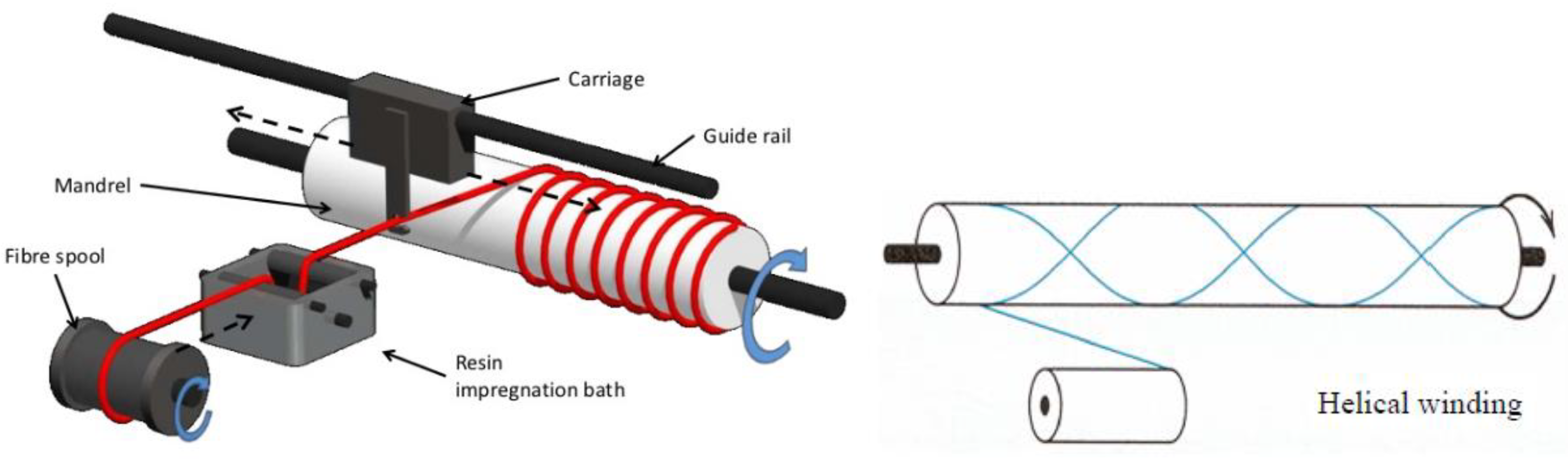
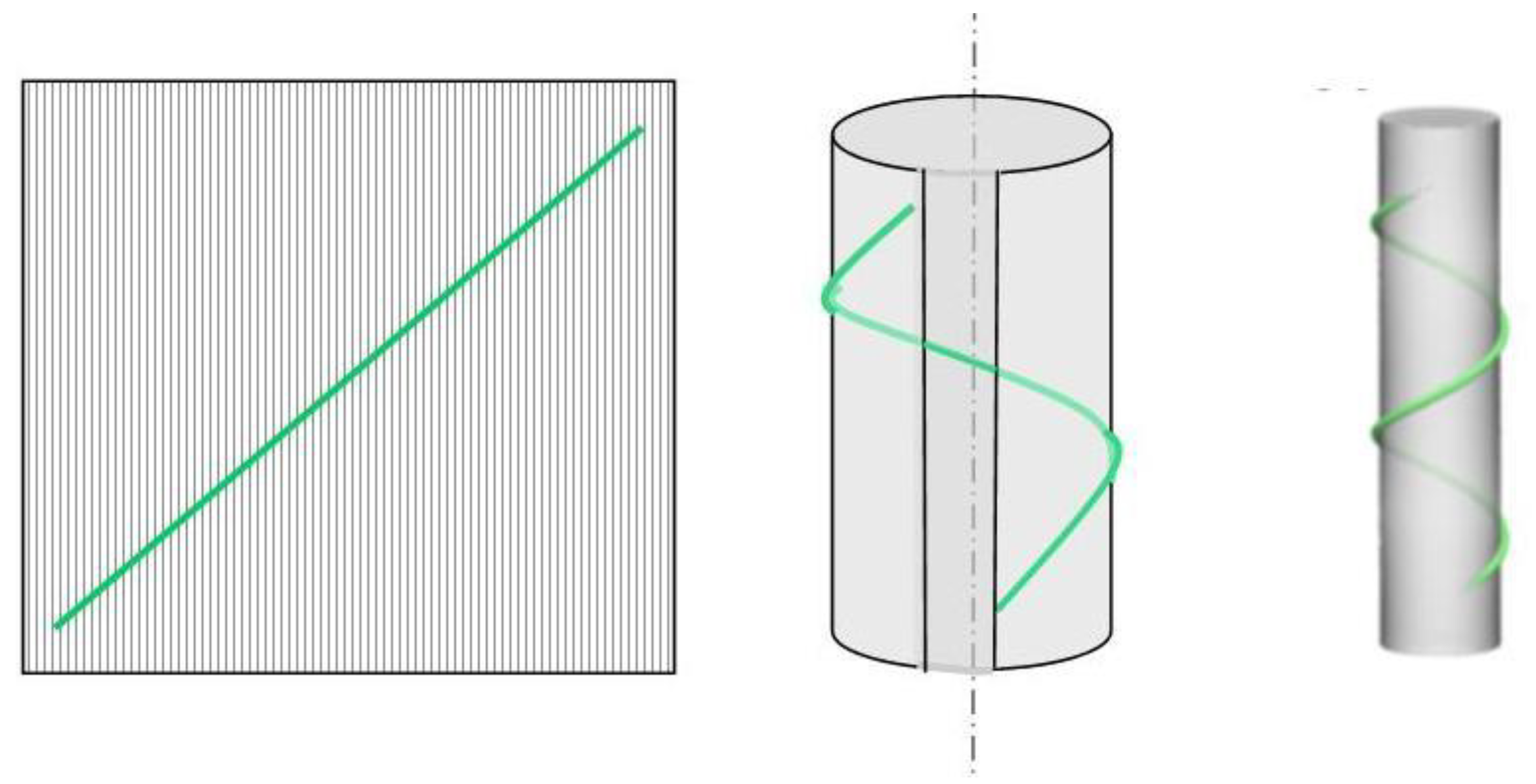
The starting point in identifying the optimum winding angle is the use of certain mathematical tools, such as the geodesic path principle, which is one of the main principles employed in filament winding. A line segment (the shortest distance between two points) wrapped onto a right-angle cylinder is a geodesic arc, i.e., the shortest path around a cylinder (see Figure 3). This is true no matter how tightly the cylinder is rolled (decreasing the radius r). The profile of a geodesic arc on a right circular cylinder is a function of arcsine, i.e., sin−1, which is a part of a circular helix. This definition is useful in filament winding, since the fibres will follow the shortest path on the mandrel surfaces between any given two points. Logically, the geodesic arc is a stable path, as the fibres would have to stretch to deviate from the set path. On a cylinder, the geodesic arc is a helical path with a constant winding angle, α. This means that in order to wind the end points of a cylinder, the geodesic path cannot be followed completely. A change in the winding direction is required to generate a complete layer, where this deviation from the geodesic path ensures that the fibres stay in place through friction [7].
When the geodesic principle is utilised, any point on the geodesic arc of an axisymmetric mandrel satisfies [8]:
r sin(α) = constant
where r is the radius of the cylinder and α is the winding angle, which represents the orientation of the fibre with respect to the axial direction of the cylinder. When helical winding is used, as in the current study, the winding angle varies between 5° and 85°. Depending on this angle, the mandrel might rotate several times before the fibres have traversed the whole circumference of the mandrel and start laying adjacent to the previous winding. This provides a pattern of alternating positive and negative winding angles, with each layer forming a two-ply layup of [α/−α].

2.2. Material and Boundary Conditions

The various mechanical properties of the utilised glass fibre composite material in the current study are summarised in Table 1. These properties were measured through mechanical testing at Swansea University during the course of the current project. As would be expected, the Young’s modulus in the X direction (longitudinal) is higher than that in the Y and Z directions (transverse). This also applies to the other mechanical properties such as the shear modulus, tensile strength, and Poisson’s ratio, as shown in the table.
A sub-structure modelling technique was utilised to allow the analysis of the (float) model and the solid (anchoring system) model to assess the stress levels in the laminate that was built utilising the filament winding approach. The plate of the support, which is connected to a stainless steel cable, was embedded between the plies of the top and bottom shells. The contact boundary condition of the plate with the top and bottom shells was assumed to be frictionless in order to reduce the number of uncertain parameters, as well as to minimise the modelling time and cost. The “ribs” that surround the float were assumed to be circumferential around the body of the float system. The cables utilised in the model were assumed to be made of stainless steel, with fixed supports assumed at the end of the cables. In order to simplify the analysis of the geometry, one quarter of the float was modelled by applying symmetric axis boundary conditions. These conditions assume that as long as the float is symmetric along the three employed axes, one-quarter is sufficient to simplify the problem, as well as to generalise the solution. This makes the analysis significantly more efficient and applicable to the whole geometry.

2.3. Multi-Level Optimisation Strategy

One of the major aims of the current study is to determine the optimum thickness of the filament-wound composite top and bottom shells that support the stainless steel plate, as shown in Figure 4. Moreover, the sequence for the filament winding angle orientations of the plies is also required to ensure that the highest possible strength of the structure is attained. This requires the optimum combined solution for the thickness and filament winding angle orientations that provide the highest supportive strength to the float system.
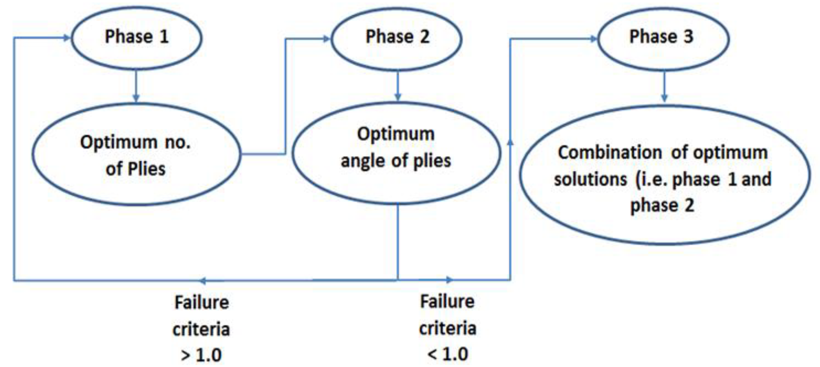
Thus, the design variables of the system consist of the stacking sequence in terms of angle orientations, as well as the number of plies in the top and bottom shells used to support the structure. The optimisation process of the float system can be divided into three successive phases that involve the thickness of the top and bottom shells, as well as the stacking sequence of the plies, as shown in the flow diagram of Figure 5.
In this analysis, the Tsai–Wu failure theory is applied to the composite material structures to estimate the remaining life of the material under various loading conditions [9]. The Tsai–Wu failure criterion with a high safety limit is widely applied to composite materials. This approach allows the sensitivity of each shell to be investigated and for the inverse reverse factor (IRF) to be studied, which is given by [9,10]:
I F R   =   Ultimate   applied   load Ultimate   strength
where the ultimate applied load is the maximum allowable load imposed on the structure, whereas the ultimate strength is the maximum load that the material can withstand prior to fracture. If the value of IRF is below 1, then the applied load is below the ultimate strength of the material, which indicates that the structure is safe. Whereas when the value of IRF is above 1, the applied load is beyond the material’s strength, which means that the structure is unsafe, i.e., failure is likely. The various phases for the analysis are:
Phase 1. 
The minimum number of plies for the top and bottom shells
This phase starts by assuming that the fibre orientation for all plies is 90°. This assumption will provide the best option to hold the stainless steel supports in place. This stems from the fact that when the stainless steel cables are under tension, they will try to pull the stainless steel support that resides within the plies. This action will result in pure tension in the uni-directional orientation of the fibres, which are assumed to be 90° filament-wound. This will provide a coherent and strong design for the float, with the minimum number of plies used to start the process and simplify the solution. The Tsai–Wu failure criterion is employed at this stage and solutions with IRF < 1.0 are considered for the next phase.
Phase 2. 
The optimum stacking sequence, i.e., fibre orientations
At this stage, the thickness of the top and bottom plies is kept constant while varying the stacking sequence of the fibres during filament winding. The angles start with [5°/85°] and [−5°/−85°] stacking sequences, which means that the optimum solution is within this range of angles. The reason for this selection is that angles between 0° and ±5° result in “planar” winding rather than “helical” winding, which are best suited to support the heads, domes, or caps and are beyond the scope of the current study. Additionally, angles above 85° are closer to “hoop” winding, which is been explored in the current study, since the “helical” design is the major focus of the present investigation, as recommended by Marine Power Systems (MPS). The Tsai–Wu criterion is again employed and fibre orientations with IRF < 1.0 are considered for the final stage of the optimisation process.
Phase 3. 
The optimum combination of plies vs. stacking sequence
In this phase, a 3D surface response is created in order to evaluate the combined effects of the stacking sequence and the ply thickness. The optimum solutions for phases 1 and 2 with the minimum IRF values are combined at this stage. Again, the Tsai–Wu failure criterion is employed to find the minimum combined IRF value of the stacking sequence alongside the ply thickness, which ensures the highest level of safety in the structure.

2.4. Uncertainty and Robust Design Procedure

The probability distribution of the possible solutions was obtained from the fact that there are 16 possible angles in the (+) direction and 16 possible angles in the (-) direction, given that the angles are within the range of 5° to 85° (with 5° increments). This gives a total 256 combined possible solutions for the stacking angles (162 = 256 solutions). The reason for the 5° increments is that in real-world situations, filament winding processes are restricted to winding the fibres at angles of 0°, 5°, 10°, 15°, 20°,…….., 90°. These input values of the stacking sequence were manually input into the innovative model that was developed at Swansea University. Through this, ANSYS Workbench was linked via MATLAB utilising the developed and in-house written code. The code automatically operates ANSYS, runs the model, retrieves the results, and continues to obtain the remaining sets of results. This reduces the effort, time, and number of trials used to choose the optimum design parameters for any given design. The framework for robust design proposed and employed by the authors has recently been published elsewhere, although for carbon fibre composite materials bonded via aluminium joints [11]. For the optimum and robust design, the blind kriging approach [12], a typical meta-model process, was utilised in the analysis. This approach provided outstanding results with a minimal amount of variation. This facilitated the construction of the response surfaces for each stage in the analysis, from which the optimum and robust design parameters were determined. The strategy used to optimise the uncertain parameters and the robust design starts by assuming that a certain number of plies are oriented at 90° to provide the maximum possible strength while optimising the number of plies, which is the first phase. This reduces the risk of failure of the glass fibre material. The optimum number of plies will then be taken into the second phase to obtain the best angle combinations of the filament-wound fibres. At this stage, the number of plies is kept unchanged while optimising the fibre orientation so that the likelihood of failure is eliminated. The third phase optimises the number of plies and the fibre orientations in order to obtain the best performance, i.e., maximum strength and no failure. This exercise provides a procedure that can be applied to any engineering application that involves more than a single variable through the employment of 3D response surfaces that are able to define the safest operational region.

2.5. Meta-Model Design Optimisation

In industrial practice, the optimisation of complex engineering problems is becoming increasingly popular utilising meta-model based approaches. This is due to the fact such methods reduce the burden of computationally expensive simulations. The meta-model-based optimisation relies on building a surrogate model, i.e., a meta-model, based on a reduced number of simulations, after which the model is used for optimisation purposes [13]. An approximate relationship is developed by the meta-model between the design variables and the output variable, e.g., y = f ( x 1 , x 2 ,   x n ) , where y is the output variable and x 1 , x 2 ,   x n are the input variables. This process can provide an optimised solution more quickly when the surrogate model is utilised and is less expensive to execute compared to the corresponding deterministic simulations. The “response surface” is commonly used to present the results, with a linear model being the simplest form, where the functional relationship f ( x 1 , x 2 ,   x n ) is approximated by a linear function of the design variables. On the other hand, higher order response surfaces (e.g., polynomial models) can be employed, in which the response surface is a polynomial function of the design variables. The linear or polynomial response functions are developed by minimising the sum of the squared distances from the response surface for given set of data points, i.e., the ordinary least squares approach. In this respect, the surrogate modelling approach assumes that all errors obtained from the ordinary least squared approach are normally distributed with a defined mean and variance. This assumption is often only approximate in real-world problems.
The most widely used meta-model approach is known as the “kriging” or the “Gaussian interpolation” method. The surrogate model is assumed to be capable of approximating the deterministic noise-free data and is used for high level optimisation, design space exploration, sensitivity analyses, visualization, and prototyping [14]. The additional advantage of using the kriging approach compared to the conventional least squares method is that the model goes through each data point. This allows the model to describe the uncertainty of the interpolation outside the given range of data points [15]. The kriging method is favourable compared to other techniques due to the fact that it is able to approximate complex response functions with less restrictive assumptions on the distribution of residual errors [16].

2.6. The Ordinary Kriging Model

The kriging approach is normally pre-fixed with various names, depending on the form of the function utilised in the regression analysis. In this context, the simple kriging method assumes a constant function, i.e., f(x) = 0. However, the ordinary kriging method assumes aconstant function, f(x) = 0. For more complex processes, the trend functions can be linear or quadratic, with the universal kriging model utilising a multi-variate polynomial of the form:
f ( x ) = i = 1 p α i b i ( x )
where b1(x), b2(x), …, bp(x), are the basis functions (i.e., the basis polynomials) and αi = (α1, α2, …, αp) denote the coefficients. In this approach, the regression function reproduces the general trend in the data (i.e., the largest variance), after which a Gaussian process is used to interpolate the residuals.

2.7. The Blind Kriging Model

In contrast, the blind kriging approach assumes a trend function f(x) that is unknown and difficult to determine for a given problem. This offers the possibility of identifying the most reasonable interactions within the data points [12]. This method determines the most efficient functions or features that capture the most observed variance in the sample. In an ideal scenario, the data is represented fully by a chosen trend function. The main idea is to choose new features in addition to the existing features that can be included in the kriging regression function to improve the results. The linear model that incorporates a whole set of candidate functions is:
g ( x ) = i = 1 p α i b i ( x ) + i = 1 t β i c i ( x )
where t is the number of candidate functions. The first term in this equation is the kriging regression function, where the values of the coefficient are determined independently relative to βi = (β1, β2, …, βt). The second term involves the parameters that are estimated based on the relevance of the candidate features. The estimation of the parameters, i.e., the least-squared solution, is a straightforward approach that can help to rank the features.

2.8. The Co-Kriging Model

The co-kriging approach is considered a special case of the multi-output or multi-task Gaussian process. This method exploits the correlation between coarse and fine model data to improve the predictive capability and accuracy [17]. The co-kriging model can be interpreted as the sequential construction of two kriging models—the first Kriging model is related to the coarse data and the second Kriging model is related to the residuals of the coarse data. In other words, this model employs a small set of short-term characteristics in order to predict the long-term characteristics. This, in turn, reduces the time and cost associated with generating such long-term characteristics and can provide predictions both within and outside the assumed range of characteristics.
In the current study, the ordinary, blind, and co-kriging approaches were employed in order to determine the optimum regions of the bond strength in the current case study. The study aims to validate existing data, as well as provide information on the optimum and robust design parameters. In essence, these models attempt to find the surrogate model that simulates the problem using less strict assumptions about the residual errors [18].

3. Results and Discussion

3.1. Phase 1 Results (Number of Plies of Top and Bottom Shells)

The obtained results from the blind kriging approach for phase 1 analysis are summarised in Figure 6. The mean squared error of the leave-out cross-validation was chosen to evaluate the quality of the fit, as well as the predictive capability of the technique. The blind kriging results in Figure 6a show a very good fit capability for the data through the response surface, with data showing low IRF values (below 1.0), which is desired to ensure the safety of the structure. The major outcome is the combined optimisation of the number of plies for the top and bottom shells, as shown by the data having IRF values < 1.0. The contour plot in Figure 6b more clearly shows the safety regions with IRF < 1.0, which are provided when the number of top plies is between 10 and 31 and the number of bottom plies is between 23 and 31. In other words, the bottom shell will have more severe stress and possible damage than the top shell. As indicated in Figure 6b, the minimum acceptable number of plies for the top shell is 10, whereas the minimum acceptable number of plies for the bottom shell is 23, which means that more layers are required for the bottom shell when compared to the top shell to overcome the exerted forces. On the other hand, the variance plot (Figure 6c) shows the quality of the fit, which is excellent in most regions using the blind kriging approach.
The results in the acceptable range, i.e., IRF < 1.0, are summarised in Table 2. Additionally, the IRF values are much more sensitive to the number of bottom plies when compared to the top plies. In this table, smaller IRF values result in a better optimisation of the structure. It can be seen that by increasing the plies of both the top and bottom shells, a better and safer design of the float system is obtained. This is logical, since the thicker the shell, the higher the resistance against deformation under the applied loading conditions. The minimum acceptable number of plies is 10 plies for the top shell and 23 plies for the bottom shell, which shows the more severe loading on the bottom shell when compared to the top shell. Additionally, the IRF values are much more sensitive to the number of bottom plies when compared to the top plies.
This variation in the number of plies for the top and bottom shells is due to the fact that the type of loading on the bottom shell is compressive, while it is mostly tensile on the top shell when the stainless steel cable is trying to pull the supports away from the body of the float. Since composite laminates have a significantly lower compressive strength than tensile laminates [19], the bottom shell under compression must have more plies than the top shell under tension. This means that the bottom layers will suffer more than the top layers under such loading conditions. However, choosing the highest number of plies for the top and bottom shells is impractical from cost and weight perspectives. This has to be optimised in the following stages of the optimisation process. The next phase will optimise the stacking sequence, i.e., fibre orientations, based on the minimum acceptable number of plies (10 for the top and 23 for the bottom). This number of plies will remain unchanged during the winding angle optimisation process (i.e., phase 2) to ensure that the filament winding angle is optimised while keeping the number of plies constant.

3.2. Phase 2 Results (The Fibre Stacking Sequence)

At this stage of the analysis, the stacking sequence has a fixed set of angles ranging between 5° and 85° (in the + and − directions), which gives 256 possible solutions. The top shell was assumed to have a thickness of 4.3 mm (10 plies @ 0.43 mm ply thickness, as given by the supplier), whereas the bottom shell was assumed to have a thickness of 10.08 mm (23 plies @ 0.43 mm ply thickness). In the analysis, the Tsai–Wu criterion approach along with the blind kriging fitting method were employed in order to obtain the optimum stacking sequence for the fibres. The obtained results of this phase are shown in Figure 7. It can clearly be seen from the blind kriging results in Figure 7a that this fitting approach had very good representation capability for the data, as shown by the surface response. The plot shows the minimum IRF value (i.e., below 1.0), characterised by its “valley” shape, which contains the optimum design solution to the problem. The optimum solution can be viewed more clearly in Figure 7b, i.e., the contour plot, where the optimum solution lies somewhere between +50° to +85° (value of α) and −60° (value of β), with IRF values < 1.0. The variance plot in Figure 7c shows very good quality fitting, as shown by the minimal amount of variation for most regions.
The obtained results in Figure 7 are summarised in Table 3 to find the best combination of filament winding angles with the lowest possible IRF value. It can be clearly seen that the +60°/−60° combination is the optimum solution to the problem.
In order to find a possible explanation to this stacking sequence, a simple structural analysis of the load and the floating system was performed. Based on the geometry and specifications from the manufacturing company, the angle between the load and the float system was specified as 60°. In other words, the tensile load in the stainless steel cable will be resisted by the filament-wound fibres that are aligned in the same direction as the tensile load, as shown in Figure 8. This explains the optimised solution obtained in the analysis, which was the +60°/−60° combination. However, the angle of the (+) orientation might vary between +50° and +85° due to the actual motion of the waves in reality. In other words, the stainless steel cable might be inclined at 60° on a certain occasion and then at 80° at another time. This variability explains the previous results shown in Figure 8, wherein the value of the (+) fibre orientation showed acceptable IRF results in the range of +50° to +85°.

3.3. Phase 3 Results (Number of Plies vs. the Stacking Sequence)

According to the Tsai–Wu failure criterion and the IRF values for phases 1 and 2, the analysis has shown that the bottom shell is more sensitive to the applied load than the top shell of the float system. Moreover, phase 2 has shown that the optimum combination of angles lies between +60° and −60°. At this stage, the combined solution of phases 1 and 2 for an optimum design is shown in Figure 9. In this figure, the combined angle–ply thickness optimum solution can be defined (for the ±60° winding angles). Moreover, the vertical axis presents the combined thickness (i.e., the bottom plus the top shell). From this total thickness of the float, the individual thicknesses of the top and bottom shells can be determined. For instance, if the circled point is taken as an example, the thickness of the float at this point is 14.38 mm. This represents the minimum acceptable thickness of the wall of the float, i.e., the top and bottom shells together. As discussed earlier in Section 3.2, the minimum acceptable thickness of the bottom shell is 10.08 mm, whereas that of the top shell should be at least 4.3 mm. The summation of the two thicknesses gives the thickness of the circled point in Figure 9, i.e., 14.38 mm, which is the worst case scenario. At this particular point, the optimum thickness and ply angle orientation are obtained, giving a reduced IRF value of 0.89 (an improvement of 10% in terms of safety when compared to the original case of phase 1). This is applicable to any point on this graph, which allows the designer to choose the number of plies for the top and bottom shells, taking into consideration the minimum allowable number of plies for each shell. This solution to the float system problem is comprehensive and applicable to the investigated design for an optimum solution for the number of plies and filament winding angles.

4. Conclusions

This study has provided a full-scale investigation of the proposed MPS float system, which is to be manufactured from glass-reinforced plastic (GRP). This case study has allowed the implementation of the developed code at Swansea University to link ANSYS Workbench through MATLAB in order to generate a set of data that can be studied using uncertainty models. The study has revealed the optimum filament winding angle, as well as the optimum thicknesses of the top and bottom shells of the float system in terms of the number of plies from which each shell is constructed. The optimum set of filament winding angles is ±60°, which is in agreement with the applied load in the cable, which was specified by the manufacturer to be inclined at 60° relative to the float system. Furthermore, the optimum number of plies that provided a safe structure under the applied loads was also obtained. The combined solution provides a set of thickness values from which the designer can choose the optimum thickness for a certain geometry, taking into account the weight and cost of construction. This analysis is a useful exercise that can be applied to any engineering structure that involves more than a single uncertain parameter in the final design. This reduces the modelling time and the involved costs when the optimum range of properties is defined. This also provides the starting point for the design and manufacture of components for any engineering application. A new innovative technique that is not available in ANSYS was employed so that the number of layers and the fibre orientation could be simulated simultaneously while providing the optimum design requirements.

Author Contributions

Investigation, Validation and Writing, N.A.; Methodology and Software, C.G.; Writing—Review and Editing, Z.A.; Resources and Supervision, F.B.; Supervision and Conceptualisation, H.H.K.; Writing—Review and Editing, M.I.F.; Funding Acquisition, J.S. All authors have read and agreed to the published version of the manuscript.

Funding

This research was funded by the Advanced Sustainable Manufacturing Technologies (ASTUTE 2020) project based at Swansea University. The ASTUTE 2020 project is funded by the European Regional Development Fund through the Welsh Government and the Welsh European Funding Office (WEFO). Furthermore, Dr Cinzia Giannetti acknowledges the support of the UK Engineering and Physical Sciences Research Council (EPSRC) project EP/S001387/1 towards the publication of this paper.

Conflicts of Interest

The authors declare no conflict of interest.

Replication of Results

This is possible utilising the published data in the current article. However, the MATLAB code is owned by Swansea University under copy right protection and cannot be made available. However, open calls to the research community to collaborate on various projects by providing data to Swansea University for a joint publication are more than welcome. Please get in touch with the corresponding author for future collaborative projects.

References

  1. IRENA. IRENA Ocean Energy Technology Brief Wave Energy; IRENA: Abu Dhabi, UAE, 2014. [Google Scholar]
  2. Rosato, D.V.; Grove, C.S. Filament Winding: Its Development, Manufacture, Applications, and Design (Polymer Engineering and Technology); Interscience: New York, NY, USA, 1964. [Google Scholar]
  3. Zu, L. Design and Optimization of Filament Wound Composite Pressure Vessels. Master Thesis, TU Delft, Delft, The Netherlands, 2012. [Google Scholar]
  4. Chen, F.C. A filament wound structure technology overview. Mater. Chem. Phys. 1995, 42, 96–100. [Google Scholar]
  5. Onder, A.; Sayman, O.; Dogan, T.; Tarakcioglu, N. Burst failure load of composite pressure vessels. Compos. Struct. 2009, 89, 159–166. [Google Scholar] [CrossRef]
  6. Sulaiman, S.; Borazjani, S.; Tang, S.H. Finite element analysis of filament-wound composite pressure vessel under internal pressure. In IOP Conference Series: Materials Science and Engineering, Proceedings of the 2nd International Conference on Mechanical Engineering Research (ICMER 2013), Kuantan, Pahang, Malaysia, 1–4 July 2013; IOP Publishing: Bristol, UK, 2013. [Google Scholar]
  7. Skjærholt, I. Integration Tools for Design and Process Control of Filament Winding; Norwegian University of Science and Technology: Trondheim, Norway, 2012. [Google Scholar]
  8. Liu, P.; Chu, J.; Hou, S.; Xu, P.; Zheng, J. Numerical simulation and optimal design for composite high-pressure hydrogen storage vessel: A review. Renew. Sustain. Energy Rev. 2012, 16, 1817–1827. [Google Scholar] [CrossRef]
  9. Paknahad, A.; Fathi, A.; Goudarzi, A.M.; Nourani, R. Optimum head design of filament wound composite pressure vessels using a hybrid model of FE analysis and inertia weight PSO algorithm. Int. J. Mater. Form. 2016, 9, 49–57. [Google Scholar] [CrossRef]
  10. Tsai, S.W.; Wu, E.M. A General Theory of Strength for Anisotropic Materials. J. Compos. Mater. 1971, 5, 58–80. [Google Scholar] [CrossRef]
  11. Aldoumani, N.; Khodaparast, H.H.; Cameron, I.; Friswell, M.; Jones, D.; Chandrashaker, A.; Sienz, J. The robustness of carbon fibre members bonded to aluminium connectors in aerial delivery systems. Cogent Eng. 2016, 3, 1225879. [Google Scholar] [CrossRef] [Green Version]
  12. Guyon, I.; Elisseeff, A. An introduction to variable and feature selection. J. Mach. Learn. Res. 2003, 3, 1157–1182. [Google Scholar]
  13. Gano, S.E.; Renaud, J.E.; Martin, J.D.; Simpson, T.W. Update strategies for kriging models used in variable fidelity optimization. Struct. Multidiscip. Optim. 2006, 32, 287–298. [Google Scholar] [CrossRef]
  14. Booker, A.J.; Dennis, J.E., Jr.; Frank, P.D.; Serafini, D.B.; Torczon, V.; Trosset, M.W. A rigorous framework for optimization of expensive functions by surrogates. Struct. Optim. 1999, 17, 1–13. [Google Scholar] [CrossRef]
  15. Ulaganathan, S.; Couckuyt, I.; Dhaene, T.; Laermans, E.; Degroote, J. On the use of gradients in Kriging surrogate models. In Proceedings of the Winter Simulation Conference 2014, Savannah, GA, USA, 7–10 December 2014; IEEE: New York, NY, USA, 2014. [Google Scholar] [CrossRef] [Green Version]
  16. Martin, J.D.; Simpson, T.W. A study on the use of Kriging models to approximate deterministic computer models. In Proceedings of the DETC’03 ASME 2003 Design Engineering Technical Conferences and Computers and Information in Engineering Conference, Chicago, IL, USA, 2–6 September 2003. [Google Scholar]
  17. Kennedy, M.C.; O’Hagan, A. Predicting the output from a complex computer code when fast approximations are available. Biometrika 2000, 87, 1–13. [Google Scholar] [CrossRef] [Green Version]
  18. Couckuyt, I.; Forrester, A.; Gorissen, D.; De Turck, F.; Dhaene, T. Blind Kriging: Implementation and performance analysis. Adv. Eng. Softw. 2012, 49, 1–13. [Google Scholar] [CrossRef] [Green Version]
  19. Liu, D.; Fleck, N.A.; Sutcliffe, M.P.F. Compressive strength of fibre composites with random&bre waviness. J. Mech. Phys. Solids 2004, 52, 1481–1505. [Google Scholar]
Figure 1. The floating device in the energy harvesting system.
Eng 01 00008 g001
Figure 2. The working principle of the helical filament winding process.
Eng 01 00008 g002
Figure 3. An illustration of the geodesic path on a cylindrical surface.
Eng 01 00008 g003
Figure 4. The stainless steel support with the top and bottom plies of the filament-wound composite.
Eng 01 00008 g004
Figure 5. The multi-level optimisation strategy.
Eng 01 00008 g005
Figure 6. Phase 1: Optimising the number of plies: (a) the blind kriging response surface; (b) the contour plot; (c) the variance plot.
Eng 01 00008 g006
Figure 7. Phase 2: Optimising the ply orientation: (a) the blind kriging response surface; (b) the contour plot; (c) the variance plot. Note: All angles are in degrees (°).
Eng 01 00008 g007
Figure 8. A simple structural analysis explaining the optimum +60°/−60° combination of the optimum stacking sequence. Note: All angles are in degrees (°).
Eng 01 00008 g008
Figure 9. The combined solution for the thickness of the float (the top and bottom shells) at the optimum filament winding angle of ±60°.
Eng 01 00008 g009
Table 1. The experimental properties of the glass fibre material (Swansea University).
Material PropertiesValue
Young’s Modulus X direction28,000 MPa
Young’s Modulus Y direction6900 MPa
Young’s Modulus Z direction6900 MPa
Poisson’s Ratio XY0.3
Poisson’s Ratio YZ0.19
Poisson’s Ratio XZ0.19
Shear Modulus XY11,100 MPa
Shear Modulus YZ2980 MPa
Shear Modulus XZ2980 MPa
Tensile Strength X direction1100 MPa
Tensile Strength Y direction35 MPa
Tensile Strength Z direction35 MPa
Table 2. A summary of the inverse reverse factor (IRF) values obtained for the shell optimization *.
Top Plies #Bottom Plies #IRF Values
30310.6160867
26300.6853152
22310.6944406
28290.6949207
29280.7232109
24290.7396711
20300.7493208
18300.790386
31260.7919314
25270.8047401
21280.8076068
27260.8297545
14310.844326
30250.8538816
23260.8634863
16290.8730014
19270.8788239
22250.914228
17270.9276962
26240.9404642
28230.984838
12290.9925366
13280.9995041
Note: * When the value of IRF < 1, this means the structure is safe, whereas when IRF > 1 the structure will fail.
Table 3. A summary of the IRF values obtained for the stacking sequence optimisation* (the first column of angles is α, whereas the second column is β).
Angle 1Angle 2IRF Values
60−600.936464153
65−600.936740126
55−600.937034556
75−600.937040329
70−600.937175776
80−600.937716612
85−600.938415852
50−600.940729225
70−650.982900049
55−650.982931364
60−650.983015988
65−650.983230577
75−650.983428191
50−650.983641761
80−650.984033312
85−650.984664912
50−550.999807636
55−660.999854478
Note: * When the value of IRF < 1, this means the structure is safe, whereas when IRF > 1 the structure will fail. All angles are in degrees (°).

