


1 Introduction
1.1 Background and motivation
Ice is a crystalline solid-state material exhibiting both ductile and brittle deformation under tensile stress loading (Schulson and Duval, Reference Schulson and Duval2009). Glaciers can be seismically active, exhibiting a variety of temporally and spatially clustered events, caused by a broad range of source mechanisms (West and others, Reference West, Larsen, Truffer, O'Neel and LeBlanc2010; Brueckl and others, Reference Brueckl, Binder, Mertl, Beer, Kougioumtzoglou, Patelli and Au2015; Podolskiy and Walter, Reference Podolskiy and Walter2016; Aster and Winberry, Reference Aster and Winberry2017). Myriad studies have linked glacial seismicity to glacier motion either directly or indirectly during the formation or deepening of crevasses, and to subglacial hydrology (VanWormer and Berg, Reference VanWormer and Berg1973; Deichmann and others, Reference Deichmann, Ansorge and Röthlisberger1979; Weaver and Malone, Reference Weaver and Malone1979; Metaxian and others, Reference Métaxian, Araujo, Mora and Lesage2003; Walter and others, Reference Walter, Deichmann and Funk2008; Allstadt and Malone, Reference Allstadt and Malone2014; Bartholomaus and others, Reference Bartholomaus2015; Vore and others, Reference Vore, Bartholomaus, Winberry, Walter and Amundson2019). In the sub-polar regions, the seasonal variation of glacier motion is closely related to the transient water input and the apparent subglacial drainage system capacity. A commonly cited model for glacier motion includes the notion that transient water input rates exceed the capacity of the subglacial drainage system, which increases the basal water pressure and results in enhanced basal motion of the glacier (Iken and Bindschadler, Reference Iken and Bindschadler1986; Anderson and others, Reference Anderson2004; Bartholomaus and others, Reference Bartholomaus, Anderson and Anderson2008; Schoof, Reference Schoof2010). The sudden ice motion can be seismogenic, producing a so-called ‘icequake’. Early passive seismological experiments on glaciers yielded insight into the nature of icequakes, interpreting the opening of surface crevasses as the main seismic source of events (Neave and Savage, Reference Neave and Savage1970). Deichmann and others (Reference Deichmann2000) reported deep icequakes from below the brittle-to-ductile transition, recorded at the Unteraargletscher (CH). Helmstetter and others (Reference Helmstetter, Moreau, Nicolas, Comon and Gay2015) deduced hydro-fracturing as seismic source mechanism of events below the brittle-to-ductile transition of a temperate glacier.
Boon and Sharp (Reference Boon and Sharp2003) observed hydrologically-driven ice fracturing on a cold, Arctic glacier which established a surface–bed connection. Rapid supraglacial lake drainage events on the Greenland Ice Sheet initiated hydrologically-driven surface–bed connections through km-thick, cold ice (Das and others, Reference Das2008; Doyle and others, Reference Doyle2013; Jones and others, Reference Jones, Kulessa, Doyle, Dow and Hubbard2013; Carmichael and others, Reference Carmichael2015; Dow and others, Reference Dow2015). These drainage events coincided with increased seismicity, transient acceleration, ice-sheet uplift and horizontal displacement. Hence, water can potentially be found at all depths of temperate, polythermal and cold-based glaciers and ice sheets, and hydrologically-driven ice fracturing is a widespread and efficient mechanism to propagate englacial and subglacial drainage systems (e.g. Fountain and others, Reference Fountain, Jacobel, Schlichting and Jansson2005; van der Veen, Reference van der Veen2007; Benn and others, Reference Benn, Gulley, Luckman, Adamek and Glowacki2009; Harper and others, Reference Harper, Bradford, Humphrey and Meierbachtol2010; Tsai and Rice, Reference Tsai and Rice2010).
The Icelandic term jökulhlaup describes a sudden release of water from a glacier, also commonly referred to as a glacial outburst flood. The discharged water can be stored in ice-marginal, subglacial, englacial and supraglacial locations, although volcanogenic and rainfall-induced floods can occur without significant water storage (Roberts, Reference Roberts2005). Jökulhlaups are an episodic, but common phenomena for glacierized regions like Greenland and span a broad range of flood volume and frequency (e.g. Tweed and Russell, Reference Tweed and Russell1999; Mayer and Schuler, Reference Mayer and Schuler2005; Weidick and Citterio, Reference Weidick and Citterio2011; Larsen and others, Reference Larsen2013; Carrivick and others, Reference Carrivick2017; Grinsted and others, Reference Grinsted, Hvidberg, Campos and Dahl-Jensen2017). The classic jökulhlaup theory (Nye, Reference Nye1976; Spring and Hutter, Reference Spring and Hutter1981, Reference Spring and Hutter1982; Clarke, Reference Clarke1982) assumes a pre-existing conduit with a constant potential gradient, which pipes the water through the glacier. Two competing processes determine the varying conduit cross-section and consequently, the proglacial discharge. Friction between floodwater and the conduit wall, as well as the initial water heat content enlarge the conduit cross-section through melting, whereas ice creep driven by the overburden pressure reduces the cross-section. Water pressure in the conduit is assumed not to exceed the ice overburden pressure. The classic jökulhlaup model reproduces proglacial discharge curves characterized by an exponential-like discharge increase over days and weeks.
The 1996 jökulhlaup of the subglacial lake Grímsvötn under the temperate Vatnajökull ice cap showed an exceptionally high maximum discharge reached in just ~16 h after the initial glacier terminus burst out (Snorrason and others, Reference Snorrason and Haraldsson1997). This rapidly-rising jökulhlaup cannot be explained by the classic jökulhlaup theory, and hydro-fracturing is assumed to be a fundamental process of this type of jökulhlaup (Roberts and others, Reference Roberts, Russell, Tweed and Knudsen2000; Flowers and others, Reference Flowers, Björnsson, Palsson and Clarke2004; Björnsson, Reference Björnsson2011). Jóhannesson (Reference Jóhannesson2002) suggested a subglacial pressure wave forcing a pathway for the subsequent floodwater discharge for the 1996 Grímsvötn jökulhlaup. A necessary condition for the pressure wave initiation is, in contrast to the classic jökulhlaup theory, a basal water pressure that locally exceeds the overburden pressure (glaciostatic stress). Several following reports showed that rapidly-rising jökulhlaups are often observed (e.g. Einarsson and others, Reference Einarsson2016, Reference Einarsson, Jóhannesson, Thorsteinsson, Gaidos and Zwinger2017), and can also occur in non-volcanic environments outside of Iceland (e.g. Grinsted and others, Reference Grinsted, Hvidberg, Campos and Dahl-Jensen2017).
Increased microseismic activity in temporal and spatial clusters is observed during jökulhlaups (Walter and others, Reference Walter, Clinton, Dreger, Deichmann and Funk2010). Walter and others (Reference Walter2009) linked the vast majority (>99%) of the detected seismic events to shallow tensile faulting due to the opening of surface crevasses for the 2004 Gornerlake (CH) jökulhlaup. Less than 0.5% of the events could be located below the crevassing zone. Moment tensor analysis yielded a tensile crack source with steeply dipping fault planes for the intermediate depth (~100 m) events, and a tensile fracturing source with a near-horizontal, bed-parallel, fault plane for the basal events (Walter and others, Reference Walter, Clinton, Dreger, Deichmann and Funk2010). Contrary to their expectation, the detected basal events correlated with decreasing and minimum basal water pressures. Walter and others (Reference Walter, Deichmann and Funk2008, Reference Walter, Clinton, Dreger, Deichmann and Funk2010) interpreted them as the collapse of cavity roofs during periods of low basal water pressure. They found no evidence that subglacial routing of the lake water caused brittle deformation radiating seismic energy during active flooding. However, the 2004 Gornerlake outburst showed rather the characteristics of a classic jökulhlaup with an exponential proglacial discharge increase over days.
In this paper, we present results of a seismic monitoring campaign during the 2012 fill-and-drain cycle of an ice-dammed lake. The lake is dammed by the predominantly cold-based A. P. Olsen Ice Cap (APO), NE-Greenland, and features a quasi-annual fill-and-drain cycle. The 2012 outburst event featured a rapidly-rising discharge and was one of the most destructive APO jökulhlaups observed so far. To our knowledge, this is the first ‘on-ice’ seismic monitoring in the path of a rapidly-rising jökulhlaup, covering a full fill-and-drain cycle. Our study aims at describing first-order observations of the spatiotemporal variation of seismicity and discusses the potential of seismic interferometry to monitor medium changes during a jökulhlaup as well as the ambiguities in interpretation. Furthermore, the relationships between seismicity and relevant environmental data (air temperature, river discharge, snow depth, precipitation) are presented and discussed.
1.2 Study site
In 1995, the Zackenberg Research Station (ZRS; 74°28′N, 20°34′W; Fig. 1) was established in the National Park of Northeast Greenland. The Zackenberg region is the longest-serving study site of the ‘Greenland Ecosystem Monitoring’ program (GEM, www.g-e-m.dk; Albon and others, Reference Albon, Thiede and Holmén2014). This high-Arctic setting has an annual mean temperature of −9.0°C (mean over 1996–2013) and experiences positive monthly mean temperatures only in June, July, August and September (data.g-e-m.dk). The mean annual precipitation is 211 mm (mean over 1996–2013), predominantly as snow during winter (Jensen and others, Reference Jensen, Christensen and Schmidt2014). Regular flood waves from jökulhlaups have been recorded for the Zackenberg river since the hydrometric monitoring at the research station was installed in 1996. River discharge is continuously measured as part of the GEM sub-programmes ClimateBasis and GeoBasis (www.g-e-m.dk). The river catchment covers 514 km2, of which, 106 km2 are covered by glaciers and ice caps (Fig. 1). The river catchment receives no discharge contribution from the Greenland Ice Sheet. Discharge data yield typical summer values in the range of 10–60 m3 s−1 (Søndergaard and others, Reference Søndergaard2015), though the episodic jökulhlaups show maximum discharges of ~100–250 m3 s−1. Generally, the jökulhlaup hydrograph is characterized by a rapidly increasing discharge over just a few hours. The whole flood event takes about half a day. The 2012 flood wave on August 6 was one of the largest observed so far, triggering substantial erosion of the riverbanks and bed. The hydrometric station was destroyed, and consequently, it was not possible to completely measure the 2012 flood discharge. The estimated 2012 peak discharge of 215 m3 s−1 is considered a minimum value (Personal communication J. Abermann).
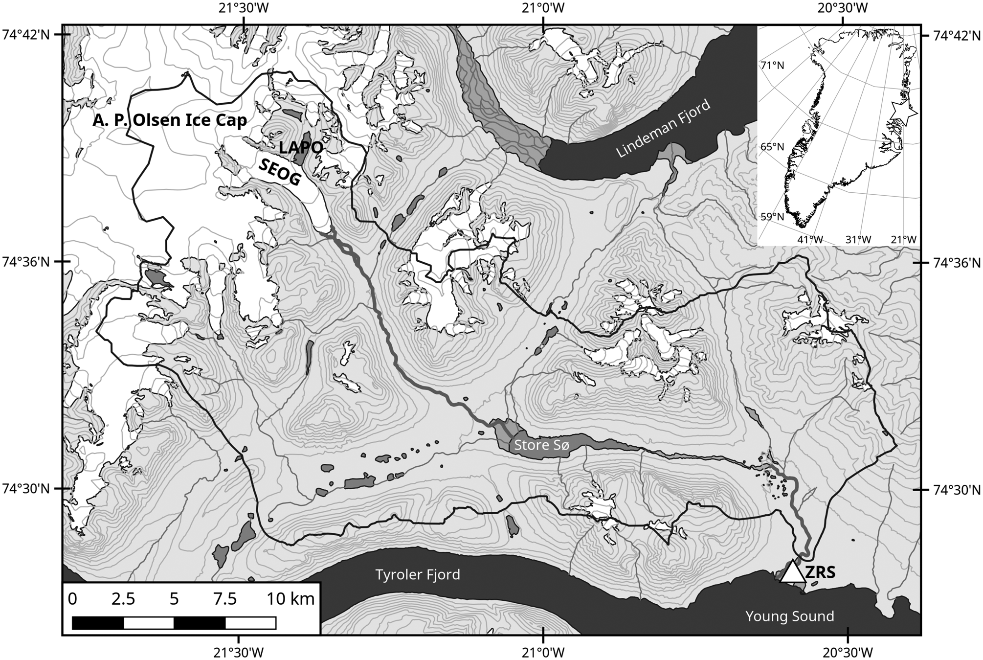
Fig. 1. The A.P. Olsen Ice Cap is ~35 km inland from the Zackenberg Research Station (ZRS, white triangle). The origin of the recurring flood waves is an ice-marginal lake (LAPO) dammed by the Southeast outlet glacier (SEOG) of the A. P. Olsen Ice Cap. On its route from the SEOG terminus to the ZRS, where the water drains into the Young Sound, the flood wave passes the Store Sø (‘Large Lake’). The black line encircles the entire river catchment basin.
Jökulhlaups originate from a marginal, ice-dammed lake, impounded by the southeast outlet glacier of the A.P. Olsen Ice Cap (APO, 74°38′N, 21°26′W; Fig. 1). The predominantly cold-based APO is a peripheral ice cap in the northeast of Greenland, ~35 km inland of the research station, exhibiting maximum ice depths of ~350 m (Binder and others, Reference Binder2013). On the occasion of the fourth International Polar Year, the GlacioBasis monitoring program (www.g-e-m.dk) was initiated in order to quantify the APO mass balance. GlacioBasis operates in total three automated weather stations (AWSs, Fig. 2) on the APO. The mean specific mass balance of ~−0.5 m w.e. correlates with an equilibrium line altitude ranging between 1100 and 1300 m a.s.l. (Larsen and others, Reference Larsen, Citterio, Hock and Ahlström2015). The southeast outlet glacier dams an adjacent, ice-free side valley (~1.5 × 0.5 km) where water accumulates and forms the lake A. P. Olsen (LAPO, Fig. 1). The lake is regularly drained by jökulhlaups with a quasi-annual cycle. The maximum lake volume varies between the individual jökulhlaup events and is in the range 8–16 × 106 m3. Generally, the lake fill-and-drain cycle starts with the melt season in May/June and ends between early July and the first months of the consecutive year. Based on the existing time series, jökulhlaups are most probable for August. On its way downstream from the APO to the research station, the river runs through the Store Sø (‘Large Lake’, Fig. 1). The lake has an area of ~4.4 km2 and likely dampens the outburst hydrograph. However, recorded discharge data at the station still show the characteristics of a rapidly-rising jökulhlaup. Since 2008 an automated camera (Fig. 2), as part of the GeoBasis program, provides one daily photograph of the lake, and thus, one inferred water-level estimate. Additionally, a pressure sensor (Fig. 2) installed in 2013 records the lake water level, showing that the 2013 and 2016 jökulhlaups started at water levels of ~27 and 40 m, respectively. However, water-level measurements from this sensor were not available for the 2012 jökulhlaup described in this paper.

Fig. 2. Seismic monitoring network (APO1-APO5) on the South East outlet glacier. Interstation arrows indicate seismic interferometry sections shown in Figure 10. AWS1, AWS2: GlacioBasis automated weather stations. The ice-dammed lake is indicated by the grey area. The GeoBasis automated camera (AC) takes one photo per day. In 2013, a pressure sensor (PS) was installed to log the lake's water depth. Contour lines of the ice thickness based on GPR data are shown (dashed grey line). Solid thick black line represents the glacier's outline, including the rock outcrop in the upper part.
1.3 Seismic monitoring network
The seismic monitoring network was installed in April 2012 when the lake water level was zero. The continuous recording seismic network consisted of five locations in the ablation zone of the outlet glacier. All sensors were installed in shallow boreholes (~3 m) and were covered with a geotextile to reduce ablation rates by up to 50% (Olefs and Lehning, Reference Olefs and Lehning2010). Two locations were designed as tripartite arrays (APO4, APO5), and the remaining three locations (APO1, APO2, APO3) were equipped with three-component sensors (Fig. 2). The tripartite arrays have a radius of 12 m and are equipped with vertical geophones. All sensors have a characteristic frequency of 4.5 Hz (Geospace GS-11D) and are attached to a Reftek 130 recorder with a sampling frequency of 500 Hz. The power supply of the monitoring stations consists of a combination of solar panels (2 × 20 Watts) and a vertical wind turbine (Leading Edge v50) charging batteries. The maximum interstation distance is 1200 m. After the installation of the monitoring network, a ground-penetrating radar (GPR) survey was conducted which found ice thicknesses in the range of 50 to 220 m for the monitoring site (Fig. 2). In 2012, the seismic network operated between May and November. All stations (APO1–AP05, Fig. 2) recorded continuously over the entire period, except for 2 d at the beginning of July.
2 Methodology
2.1 Discrete icequake analysis: event detection, classification and location
In the early pre-flood stage, only a few seismic events occur, with some expression of tremor-like events (e.g. Pomeroy and others, Reference Pomeroy, Brisbourne, Evans and Graham2013; Heeszel and others, Reference Heeszel, Walter and Kilb2014) that are characterized by a duration of up to several minutes with frequencies up to 50 Hz. Upon visual inspection, the majority of the events appeared as a sequence of body and surface waves (Fig. 3), suggesting surface crevassing as a likely possible source (e.g. Deichmann and others, Reference Deichmann2000; Mikesell and others, Reference Mikesell2012). The surface-wave peaks occur at frequencies between 5 and 30 Hz and seem to interfere with later scattered surface-wave arrivals. Different arrival times at the two horizontal components suggest the existence of both Rayleigh and Love waves. We first detect icequakes and then use a wave-type discriminator based on the waveform polarization observed at a centrally located three-component station. Results from these initial analyses suggested that a vast majority of icequakes were surface waves and so we detail a simplified 2-D location algorithm to locate sources based on the surface-wave arrival times.

Fig. 3. A typical seismic event in the syn-discharge phase (6/1/2012) recorded on the 3C-station APO3 with spectrograms on top. H1 is oriented towards the flow direction of the glacier (ca. SE), and H2 is oriented 90° clockwise to H1. The left, dashed vertical line indicates the onset of a body wave, and the dashed line on the right is aligned with the strongest positive peak in the following Rayleigh surface-wave arrival. Note that the surface wave appears earlier on the H2 component, suggesting the superposition of Love waves.
2.1.1 Event detection
In order to identify individual icequakes, we remove the GS-11D instrument response to simulate ground motion and bandpass the waveforms between 1 and 20 Hz. We implement a standard short-term average/long-term average (STA/LTA) transformation of each of the time series for each vertical component geophone in the array, with the short-term window at 2 s and the long-term window at 20 s. The ratio of STA/LTA essentially forms a new time series that triggers a possible candidate event if that transformed signal rises above a threshold of four times the median daily STA/LTA ratio and that trigger ends when the transformed signal falls below two times the median daily STA/LTA ratio. If eight sensors simultaneously trigger with the aforementioned STA/LTA thresholds, then we have a candidate event and we additionally determine the time at which each of the sensors triggered, which informs our location estimates.
2.1.2 Event-type discrimination
We arrange the trigger times relative to those sensors that triggered first and fit a line to the travel-time plotted with respect to the inter-sensor distance relative to which sensor triggers first, irrespective of the network geometry so that the distance is calculated as the distance from that sensor to the first triggered sensor. The reciprocal of the slope of the fitted line is an estimate of the apparent wave speed as the wave moves across the glacier array. A histogram of these values indicates a strong peak near ~1500 m s−1, which would be consistent with predominantly surface waves triggering our sensors. Note that the value corresponds to an apparent velocity across the array and would not be the actual surface-wave velocities, but rather close. Also, compared to other studies (e.g. Mikesell and others, Reference Mikesell2012), this velocity appears to be low. However, our interferometric analysis in the next section suggests that surface-wave velocities in that frequency range comprise the effects of both ice and basal sediments. Some of the stations comprising the network included three-component geophones (APO1–APO3). We can utilize the polarization of the waveforms to further discriminate the type and distinguish between body and surface waves. A frequency-based polarization test has also recently been utilized for a glaciological study with the so-called glaciohydraulic tremor (Vore and others, Reference Vore, Bartholomaus, Winberry, Walter and Amundson2019). For the incoming waves to the three-component station, the rectilinearity (also commonly referred to sometimes as simply ‘linearity’), dip and azimuth can be determined based on the analysis of the data within discrete windows, if the three components on the sensor are orthogonal to one another. We generally follow the methods described in Baillard and others (Reference Baillard, Crawford, Ballu, Hibert and Mangeney2014). We first compute the 3 × 3 covariance matrix across the samples with a sliding window of 0.5 s. We arbitrarily define the window length to be short enough to capture local short duration waveforms but with sufficient length for the polarization test.
Ordered eigenvalues determined from the covariance matrix are used to compute the azimuth, dip or otherwise known as incidence angle (Vidale, Reference Vidale1986), and rectilinearity (Jurkevics, Reference Jurkevics1988). We compute the azimuth, or commonly referred to as backazimuth, of the incoming seismic energy within a window by computing the arctangent of the largest eigenvalue. We refer to the azimuth portion of the polarization analysis later as it further informs directionality of the incoming waves regardless of whether we detect them with the location algorithm outlined in the next section.
Rectilinearity approaching a value of 1 would indicate a body wave. In addition, P waves would have near-vertical incidence (dip ~90°), while S waves would be polarized horizontally (dip ~0). To combine these basic physical properties into a discrimination tool, Baillard and others (Reference Baillard, Crawford, Ballu, Hibert and Mangeney2014) proposed a dip-rectilinearity function (DR) that was used to characterize whether signals were body or surface waves at sample k. The function is such that:

where ɑ is an arbitrary weight factor that we assign a value of 1.5. When we analysed the entire study time period, only ~3% of events had a DR score that would suggest the signal consists of body waves (DR>0.5). Thus, our use of the DR function informed an analysis decision to adapt a common earthquake location method in two dimensions. Figure 4 shows an example of rectilinearity (linearity), dip, azimuth and DR calculated for an arbitrary period of time when several icequakes occurred. About 420s, several signals are present with rectilinearity ~0.5 and dip near zero which results in a DR score of ~−0.5. The near-zero dip suggests either horizontally polarized S-waves or surface waves. Since the rectilinearity is not quite zero, the wave likely consists of a mix of S-wave and surface-wave polarization. The other visible icequake signals within the time period exhibit broadly similar characteristics. Thus, we conclude that most of the icequake signals consist of horizontally polarized waves, most likely surface waves.

Fig. 4. Example of polarization test on a single station with panels including linearity (rectilinearity), dip (degrees), azimuth (degrees), decision dip-rectilinearity function (DR in the text) and the three components of ground motion (m s−1) from the seismometer at AP01. All seismometers were oriented relative to the glacier flow direction. The timescale is relative to seconds since the 0100 h on 25/6/2012.
Figure 5 shows a histogram of azimuth values derived from different hours during the study time period. This suggests that most of the wave energy is polarized parallel to the station-lake direction even when there are no detectable or visible icequakes in the record. Note that the sensors were aligned along the ice flow direction so that zero degrees azimuth would effectively be pointing southeast.

Fig. 5. Histogram of the azimuth estimates from the polarization analysis at AP01 for each 0.5 s time window over an hour-long starting at the time period indicated at the top of the panel. An example of the continuous estimation of azimuth from the polarization analysis is also shown in Figure 4. The figure suggests strong clustering in ~30° and ~210°, with the exception of the bottom left panel, which is during the jökulhlaup. Hourly histograms are computed and rotated vertically for the image in Figure 12.
2.1.3 Event location
With observations of the arrival time at each station, we implement the classical iterative least-squares earthquake location inversion method, known as Geiger's method (Geiger, Reference Geiger1912). For a set of arrival times across a seismic network, Geiger's method seeks to iteratively minimize the travel-time residual between predicted and observed travel times. From linear algebra, the ordinary matrix is d = G·δm, where d is a matrix composed of relative residuals between measured and predicted arrival times. δm is a vector comprising the unknown updates to the initial model parameters, and G is the model matrix (see below). We make several simplifications to solve this problem. First, we only consider dimensions x, y and t, which are locations and origin times of the icequakes. We exclude the z dimension since we assume that the sources are located on the surface. Given an initial guess for x and y locations of the icequake and t corresponding to the origin time for the initial location guess, at each iteration we compute

where x i and y i are the coordinates of the i-th sensor, v is the velocity, which we assume to be 1600 m s−1 and m is the model matrix consisting of m = (t, x, y)T. The G matrix is composed of partial derivatives for each station-coordinate component arrival time. We simplify the i × 3 matrix below.

Assuming that m = m + δm, we solve for δm and update m at each iteration, where δm is

If we had additional phases (P and S), stations and were containing the vertical direction (z), we might iterate until the residual between the predicted arrival time and actual arrival time fell below a quality threshold. Since we have a more poorly constrained dataset, we simply iterate ten times and compute the std dev. of the station residuals to report how well-constrained the locations might be.
2.2 Seismic interferometry
In the most general sense, seismic interferometry can be considered as a process to synthesize wavefields through the correlation of other, e.g. recorded, wave fields (Schuster, Reference Schuster2009; Wapenaar and others, Reference Wapenaar, Draganov, Snieder, Campman and Verdel2010a, Reference Wapenaar, Slob, Snieder and Curtis2010b; Galetti and Curtis, Reference Galetti and Curtis2012). It allows one to reconstruct seismic waves travelling between two receiver stations by turning one of the receivers into a virtual source (Bakulin and Calvert, Reference Bakulin and Calvert2006), and thus sometimes is also referred to as empirical Green's function (EGF) retrieval. Ambient seismic noise interferometry relies on the abundance and potentially broad frequency spectrum of natural and anthropogenic sources of seismic energy. The location and origin times of these sources do not need to be known, but their spatial distribution must satisfy the stationary phase condition with regard to the receiver geometry (Snieder, Reference Snieder2004; Snieder and others, Reference Snieder, Wapenaar and Larner2006). In essence, this condition states that the travel paths from the ambient seismic noise source to the two receiver stations must be identical up to the receiver where the energy arrives first. With this condition met, the kinematic path effects outside the receiver deployment are eliminated in the correlation process. In the case of surface stations, the EGF is often dominated by surface waves (Forghani and Snieder, Reference Forghani and Snieder2010), although several studies extract body waves from dense deployments (e.g. Roux and others, Reference Roux, Sabra, Gerstoft, Kuperman and Fehler2005; Draganov and others, Reference Draganov, Campman, Thorbecke, Verdel and Wapenaar2009; Nakata and others, Reference Nakata, Chang, Lawrence and Boué2015). Therefore, surface-based seismic imaging using interferometry mostly involves the retrieval and inversion of surface-wave dispersion for shear-wave velocity models (Bensen and others, Reference Bensen2007; Behm and others, Reference Behm, Leahy and Snieder2014; Hannemann and others, Reference Hannemann2014; Cheng and others, Reference Cheng, Xia, Xu, Hu and Mi2018, Reference Cheng, Xia, Behm, Hu and Pang2019). The sensitivity of the EGF to small medium changes with time has been demonstrated in different environments and at different scales (e.g. Sens-Schönfelder and Wegler, Reference Sens-Schönfelder and Wegler2006; Nakata and Snieder, Reference Nakata and Snieder2012; Hillers and others, Reference Hillers2015a, Reference Hillers2015b; Larose and others, Reference Larose2015; Planes and others, Reference Planes2015), although the variability of the ambient noise source distribution and characteristics can challenge the interpretation of temporal subsurface changes (Tsai, Reference Tsai2009; Froment and others, Reference Froment2010; Fichtner, Reference Fichtner2014; Behm, Reference Behm2017).
The application of interferometry on glaciers on a local scale is still a novel approach and only a relatively small number of publications exist. Overviews are included in Aster and Winberry (Reference Aster and Winberry2017) and Podolskiy and Walter (Reference Podolskiy and Walter2016). The latter point out that the overall homogeneous glacial environment usually limits the generation of scattered coda waves, which are commonly used in the context of 4D interferometric monitoring (Snieder, Reference Snieder2006). Walter and others (Reference Walter2015) show how interferometry applied to selected and located events can be used to monitor seismic propagation velocity changes with an accuracy of 0.1% for glacier ice. Based on interferometry, Zhan (Reference Zhan2019) detects seismic anisotropy in surface waves during the 2008–2011 active phase of the surge-type Bering glacier. He related the seismic anisotropy to basal crevasse development during the switch from a channelized to a distributed subglacial discharge system.
Our workflow starts with cutting the continuous data of the entire monitoring period into 1 h segments and resampling to 80 Hz. Temporal normalization using Automatic Gain Control (AGC) with a window length of 0.2 s and spectral whitening in the band 1–35 Hz is applied. Finally, interferograms are calculated for all station pairs and all components (Z-Z, T-T, R-R) using cross-coherence (Wapenaar and others, Reference Wapenaar, Slob, Snieder and Curtis2010b). Transverse (T) and radial (R) components are obtained by rotating the horizontal components to the virtual source – receiver pair direction prior to interferometry. Due to the sparse station distribution with limited offset variation, we stack all interferograms in offset bins (bin size 200 m) to derive one representative virtual source gather for each component. Prior to stacking, the traces are time-shifted with a linear move-out (LMO) correction for a velocity of 1500 m s−1 to account for differential offsets within each bin. Each stacked trace is time-shifted back again with a reverse LMO, using the average of the offsets in the bin. Stacking also aims at simplifying and enhancing the subsurface response at the expense of spatial resolution. We stack causal and non-causal parts together as the different station pairs show a variable and complex pattern in terms of causal and non-causal arrivals. We also apply the same workflow to individual station pairs on consecutive 5 d intervals of continuous data to analyse the temporal variation of the interferograms.
3 Results and discussion
3.1 Seismic events
Initially, 108 795 candidate events are identified using the STA/LTA coincident trigger method described in Section 2.1.3. The temporal evolution of seismicity, expressed as a daily number of events and their amplitudes, and complementary environmental data are shown in Figure 6. Air temperature and snow depth data are from the GlacioBasis AWS2 (Fig. 2), while river discharge and precipitation data, provided by ClimateBasis and GeoBasis, are measured at the research station (Fig. 1). Based on the discharge curve from the Zackenberg river, we also arbitrarily define three time periods (pre-, syn-, post-discharge). The syn-discharge period is defined by a discharge rate larger than 1.75 m3 s−1 (June 7–September 13) and lags the 2012 melt season by ~1.5 weeks.
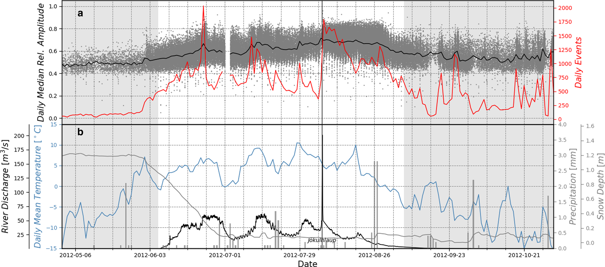
Fig. 6. Temporal evolution of seismicity. (a) Number of detected seismic events per day (red curve) and the corresponding event amplitudes (black curve; grey dots). (b) Air temperature (blue curve) and snow depth (grey curve) at station AWS2; Zackenberg river discharge (black curve) and precipitation (grey bars) at the Zackenberg research station. Grey background: pre- and post-discharge periods corresponding to a discharge <1.75 m3 s−1.
Seismic activity gradually increases closer to the first period of positive temperatures towards the end of May. In the following 3 weeks until about mid of June we observe a steadily rising number of events per day which coincides with the depletion of the snow depth. During this period, we find no significant correlation between air temperature and the number of daily events. We associate this to meltwater retention by the initially cold snow cover. Throughout the spring and early summer, the depleting snow cover becomes temperate and meltwater retention volume continuously decreases, thus steadily increasing the meltwater fraction entering the glacial system. As a consequence, basal water pressure is building up and enhances basal sliding which leads to higher surface crevassing activity and seismicity.
The period with minimum snow depth and prior the jökulhlaup (~mid of June to beginning of August) is characterized by a correlation of seismicity, air temperature, precipitation and river discharge. An increase of seismicity is observed for three pre-jökulhlaup melt events, indicated by higher river discharges, as well as for single precipitation events. We find that discharge maxima trail the seismicity peaks with a time-lag of a few (4–8) days. In this period, the river discharge shows a clear diurnal cycle.
Seismicity picks up immediately with the jökulhlaup. Afterwards, a period of ~3 weeks with larger seismic amplitudes is observed, whereas the seismicity rate (number of events per day) declines overall. Following on hypotheses proposed by Walter and others (Reference Walter, Deichmann and Funk2008, Reference Walter, Clinton, Dreger, Deichmann and Funk2010), we relate this period to the continuous collapse of the subglacial jökulhlaup drainage system. Walter and others (Reference Walter, Deichmann and Funk2008) observed a decline of seismicity for periods of high basal water pressure. They associated this observation to the buttressing effect of high water pressure in a collapsing drainage system. We can report a similar observation ~2 weeks after the jökulhlaup, where the last dominant melt event is accompanied by a drop of the seismicity rate. About three weeks after the jökulhlaup, a peak in the seismicity rate is observed which is preceded by the most intense rain event during the 2012 melt season. The corresponding seismic amplitudes remain high just until a few days after the rain event. In the following, we will discuss potential causes for the observed opposite behaviour of the seismicity rate just within 1.5 weeks.
Fudge and others (Reference Fudge, Harper, Humphrey and Pfeffer2009) reported of enhanced basal sliding rates and basal water variations initiated by an autumn rainstorm on Bench Glacier, Alaska, although equally large input events occurred in weeks prior with no apparent response. They relate this observation to the drainage system capacity decay in autumn which was intensified by the lack of water input during a 2-week period of cold and dry conditions that preceded the autumn event. In our case, the three post-jökulhlaup weeks are characterized by two competing processes. On the one hand, the gradual collapse of the channelized drainage system in the post-jökulhlaup phase decreases the drainage system capacity, whereas substantial water supply due to the positive temperatures and several precipitation events maintains an efficient drainage system. However, we suggest that besides the gradual collapse of the jökulhlaup drainage system, the water input rate is the main driver of the observed opposite seismicity rate behaviour. The melt rate is determined by a rather smooth diurnal cycle, whereas the main rain event happened in just ~3 h in the night from August 26 to 27. While the meltwater input was conveyed by the current drainage system, the rainwater input rates exceeded the capacity of the collapsing drainage system. Consequently, basal water pressure built up and led to enhanced basal sliding and the observed increase of seismic events.
3.2 Event localization
Using the 2-D location algorithm we described previously, we were able to locate several events over the duration of 2012. Because of the limited number of stations, many of the icequakes could not be located accurately and so the localization only provides guiding evidence on the nature of the icequakes and is used in the context of interpretation of interferometry. Figure 7 shows the location of the events in the pre-, syn- and post-discharge periods. The syn-discharge period is additionally split up in the times before and after the jökulhlaup. Given the network limitations and resulting large residuals, we only chose 7.5% of the events and those within the glacier for the location plot. The selection of those events is based on their time residual and amplitude. However, this restriction does not bias the average spatial distribution or clustering of the events within any of the four time periods. In the pre-discharge period (Fig. 7a), we locate 34 events within the glacier according to the selection criteria, which is in stark contrast to 7203 events during the syn-discharge period (Figs 7b, c). In the post-discharge period, 817 glacier events are present and are concentrated within the seismic network (Fig. 7d). In all periods, most of the selected events are located inside the network. Only in the syn-discharge period, we find few events propagating further south towards the centre of the glacier snout, whereas syn-discharge events after the jökulhlaup show a tendency towards the south eastern glacier snout. The black star in Figure 7 indicates the observed main floodwater exit point as observed by eyewitnesses (Gernot Weyss (ZAMG), Kirstine Skov (GeoBasis)).

Fig. 7. Locations of seismic events in the pre-, syn- and post-discharge periods. The seismic events of the syn-discharge period are separately shown for the pre- and post-jökulhlaup phase. The black star indicates the main floodwater exit point. Only the events inside the glacier boundaries and with small residuals are shown. See text for details.
3.3 Interferograms
Figure 8 shows the offset-bin stacked interferograms of all station pairs. We observe two different move-outs in the gather, e.g. a high-frequency arrival with an apparent velocity of ~1700 m s−1 and a low-frequency arrival with a velocity varying with offset. Velocities at larger offsets are ~1400–1500 m s−1, and the velocities at short offsets appear to be lower. However, the interpretation of these low-frequency arrivals is challenged at short offsets, as the sidelobes of the causal and non-causal correlation functions begin to interfere. The frequency band is limited by the Nyquist frequency (40 Hz) after resampling, but generally, we do not observe any consistent arrivals in the interferograms at frequencies larger than 30 Hz. This applies to both the stacked and pre-stack interferograms.

Fig. 8. Interferograms of all receiver pairs (entire monitoring period) in two frequency bands. All individual interferograms have been stacked in 200 m-sized offset bins. Red lines indicate linear move-out for velocities of 1700 and 1400 m s−1, respectively.
3.4. Dispersion analysis of interferograms
Dispersion analysis of surface waves retrieved through interferometry is a standard tool to analyse the depth variation of the shear-wave velocity structure. Due to the limited number of stations, we initially apply a two-station method (frequency-time analysis; Keilis-Borok, Reference Keilis-Borok1989; Bensen and others, Reference Bensen2007) to derive group velocity dispersion between station pairs. We focus on the 3C station pairs (APO1, APO2, APO3) and again stack all dispersion curves (Fig. 9) to obtain an overall view on the data. The vertical component exhibits an expected behaviour in the frequency range 3–8 Hz, but at higher frequencies, the velocities start to rise again. This is consistent with the observation in the interferograms. Velocities on the transverse component are generally higher, which qualitatively would agree with the assumption of Love waves. The radial component does not show a clear dispersion image which might result from a low H/V ratio. Based on the dispersion characteristics and bandpass filtering of the interferograms (Fig. 7), we qualitatively interpret a velocity inversion with depth as the surface-wave velocities increase with frequency. Tsuji and others (Reference Tsuji, Johansen, Ruud, Ikeda and Matsuoka2012) report a similar inverse frequency–velocity relation and associated higher surface-wave modes. They attribute it to a low-velocity layer below the base of the ice, representing unfrozen sediments. We further observe that group velocities in the low-frequency regime (3–10 Hz) are higher than the apparent phase velocities obtained from the interferograms. This reverse behaviour can appear if phase velocities increase with frequency f, as group velocities U G and phase velocities U P are related by Eqn (5) (e.g. Stein and Wyssesion, Reference Stein and Wyssesion2003):


Fig. 9. Dispersion images obtained from stacked frequency-time analysis (FTAN) of the three 3C stations (AP01, AP02, AP03) for vertical (a) and transverse (b) components, respectively. The solid black line indicates the maximum amplitude in each frequency bin.
The investigated area is well covered with GPR profiles which clearly outline the base of the ice and allow for constructing a 3-D ice thickness map (Binder and others, Reference Binder2013; Fig. 2). It shows that the area comprising the stations APO1, APO2 and APO3 has distinct ice thickness variation, such that inversion of the stacked dispersion curves might not reproduce a useful result. Therefore, we focus on individual station pairs and constrain the ice thickness in the inversion for shear-wave velocity structure based on the GPR data. We further chose to measure and invert surface-wave phase velocity to obtain more accurate shear-wave velocity model, and forward model the synthetic group velocity dispersion (Schwab and Knopoff, Reference Schwab, Knopoff and Bolt1972) and compare with the measure group velocity image. This two-step approach allows for an independent check of the obtained model based on phase velocity inversion (online Supplementary Fig. S1). Instead of using Eqn 5, we employed a two-station method (Yao and others, Reference Yao, Xu, Zhu and Xiao2005, Reference Yao, van der Hilst and de Hoop2006) to measure phase velocity. In order to acquire a reliable dispersion measurement, we applied quality control on the picked dispersion curves by requiring the interstation spacing (Δ) to be at least two times the wavelengths (λ): Δ ≥ 2λ or λ ≤ Δ/2 (Bensen and others, Reference Bensen2007; Luo and others, Reference Luo2015).
In Figure 10, we show the results for the causal part of the interferogram APO2-APO3. This profile was chosen since the base of the ice is overall flat based on the GPR measurement. Assuming a locally flat bedrock as well, Ning and others (Reference Ning, Da, Wang, Yuan and Pang2018) demonstrated that the influence on the dispersion measurement from the one-side dipping surface topography could be ignored, and the obtained shear-wave velocity model will represent an average of the structure along the profile (Luo and others, Reference Luo, Xia, Liu, Xu and Liu2009). We used a non-linear direct search neighbourhood algorithm (Wathelet and others, Reference Wathelet, Jongmans and Ohrnberger2004; Wathelet, Reference Wathelet2008), modified after Sambridge (Reference Sambridge1999) to invert phase velocity dispersion for a three-layer case. We allowed a depth variation of 90–150 m for the base of layer 1, and 110–200 m for the base of layer 2. The best-fitting model has an ice thickness of 115 m, which compares favourably to GPR data (on average 110 m along the profile). Below the ice, a thin (5 m) layer of reduced shear-wave velocity (1550 m s−1) is followed by bedrock with a shear-wave velocity of 3000 m s−1. The existence of the middle layer is further suggested by inverting for a two-layer model only, in which case the inversion got trapped in a local minimum with significantly poorer data fit and the absence of bedrock velocities (online Supplementary Fig. S2). Likewise, the horizontal components of the non-stacked interferograms had too low S/N ratio to allow the generation of a useful dispersion curve.

Fig. 10. (a) Causal part of the interferogram AP02-AP03 (vertical component, data from the entire monitoring period). (b) Phase velocity dispersion of (a). (c) Measured and inverted phase velocity dispersion curves. Colours are representing the data misfit expressed as relative RMS error. (d) Shear-wave velocity models for the dispersion curves shown in (c). The grey curve is the chosen model with the smallest RMS error.
The thin low-velocity layer possibly represents glacier till and/or poorly compacted sediments. The occurrence of basal sediments would be not surprising given the abundance elsewhere beneath the Greenland Ice Sheet (Clarke and Echelmeyer, Reference Clarke and Echelmeyer1996; Bartholomew and others, Reference Bartholomew2011; Booth and others, Reference Booth2012; Cowton and others, Reference Cowton, Nienow, Bartholomew, Sole and Mair2012; Dow and others, Reference Dow2013; Christianson and others, Reference Christianson2014; Graly and others, Reference Graly, Humphrey, Landowski and Harper2014; Walter and others, Reference Walter, Chaput and Lüthi2014; Mordret and others, Reference Mordret, Mikesell, Harig, Lipovsky and Prieto2016; Kulessa and others, Reference Kulessa, Hubbard, Booth, Bougamont, Dow, Doyle, Christoffersen, Lindbäck, Pettersson, Fitzpatrick and Jones2017). Sub-ice sedimentary layers are reported to have a wide range of shear-wave velocities, from starting as low as 200 m s−1 (Nolan and Echelmeyer, Reference Nolan and Echelmeyer1999) and up to 1500 m s−1 (Tsuji and others, Reference Tsuji, Johansen, Ruud, Ikeda and Matsuoka2012), possibly reflecting different degrees of consolidation, composition and saturation.
3.5 Time-lapse seismic interferometry and the distribution of noise sources
The continuous recording on all stations offers the possibility for interferometric time-lapse analysis. Interferograms for consecutive 5 d intervals for all station pairs are calculated using the same processing workflow as outlined in Section 2.2 (Fig. 11). In Figure 11, we show the interferogram pairs with a ‘good’ signal, which we define as relatively consistent amplitudes at realistic arrival times in at least one of the frequency bands throughout the entire monitoring period. For comparison, interferogram pairs with weak temporal coherence are shown in the online Supplementary Figure S3. In general, high seismic activity (e.g. occurrence of many events) during the syn-discharge period correlates with higher interferogram amplitudes, suggesting that the events are a contributing source of ambient seismic energy. This corresponds to the findings of Preiswerk and Walter (Reference Preiswerk and Walter2018) who identify flowing water and icequakes as contributions to mountain glacier ambient noise. In their study, they also monitor an ice-dammed lake with seismic interferometry and observe a strong disturbance of the interferograms during a 1-week long discharge period of the lake.

Fig. 11. Time-lapse interferogram sections for the station pairs AP01-AP05, AP02-AP05 and AP03-AP05 in two different frequency bands. Traces are scaled to the maximum amplitude within each section. Red lines: move-out velocities of 1400 and 1700 m s−1, respectively. Vertical grey line indicates the occurrence of the jökulhlaup at 8/6/2012. Pre- and post-discharge periods correspond to measured discharge rates <1.75 m3 s−1. See text for details.
We use the causal and non-causal characteristics of the interferogram gathers for a qualitative analysis of the dominant ambient noise sources. Of the ten station pairs, three (APO1-APO5, APO2-APO5, APO3-APO5) show relatively consistent amplitudes of the main surface-wave phases throughout the entire monitoring period. Therefore, we interpret the contributing ambient noise sources of these three station pairs to be less influenced by the temporal variation of close-by seismicity. The station pairs APO1-APO5 and APO3-APO5 have orientations roughly perpendicular to the local flow direction of the glacier while station pair APO2-APO5 has an oblique orientation relative to the flow direction. The apparent velocities in the frequency band 3–10 Hz are slow, e.g. in the range 1400–1450 m s−1. Station pair AP02-AP05 is more consistent in the causal part, indicating sources towards the north. AP03-AP05 is dominated by non-causal arrivals, which implies that the ambient energy is arriving at AP05 first. Assuming the same source region as for APO2-APO5, we suggest that the non-causal arrivals at APO3-AP05 are generated from surface waves being reflected and back-scattered at the southwestern rim of the glacier. Scattering and reflections of surface waves are a known phenomenon in exploration scale and regional seismology (e.g. Stich and Morelli, Reference Stich and Morelli2007; Halliday and others, Reference Halliday2010), and with respect to the orientation of APO3-AP05, the southwestern glacier bed rim is favourably oriented to constitute a secondary stationary-phase source for primary energy originating in the north. Station pair AP01-AP05 has both causal and non-causal arrivals, but with lower velocities compared to the two other station pairs. A possible explanation is the small offset-to-wavelength ratio which may cause interference of causal and non-causal sidelobes of the correlation function, and as such distort the interferogram. In the frequency band 10–25 Hz, higher velocities (~1700 m s−1) are observed on all three station pairs. The temporal variation of the main phases in the interferograms is discussed in more detail below. Phase velocities of interferogram pairs with low temporal consistency (Fig. 9) are partly similar, but those phases cannot be identified during the entire monitoring period. The only robust insight from these station pairs is evidence for high-frequency noise sources towards the northwest during the syn-discharge period. The earlier arrivals at these pairs point towards non-stationary sources in the sector between North and East.
A time-variable distribution of noise sources will change the interferograms. The surge in seismic activity during the syn-discharge period does not change the average spatial distribution of the located events. This maybe explains why the ballistic part of the EGF appears stable. The ballistic part of a wave describes the first arrival of a specific phase, while the coda part refers to the later arrivals caused by scattering of the same phase. Arrivals prior to the ballistic part indicate contributions from non-stationary sources, and indeed they are much more pronounced in the syn-discharge period. In order to analyse the contribution from such non-stationary sources, we take advantage of the event detection results. We define 2 s long time windows around the origin time of the detected events and mute all pre-processed data within these time windows prior to the interferometry. We compare the result with the non-muted dataset and find that there is virtually no difference in the time-lapse gathers in the frequency range of interest (3–25 Hz). On the other hand, the lack of significant coda waves possibly points towards the absence of consistent scatters at an appropriate length scale.
We therefore use the ballistic part of the EGF close to the expected arrival time as a proxy to an apparent velocity of the surface waves at the station pairs APO1-APO5, AP02-APO5 and APO3-APO5 (Fig. 12). Depending on which part is the most consistent throughout the entire monitoring period, we chose either the causal or acausal section and the frequency band, accordingly. By knowing the offset between the stations, we convert the time axis to apparent velocity and pick velocities at the maximum amplitude close to the expected surface-wave arrivals. For each section, the average apparent velocity is calculated from the mean of all velocity picks, and the apparent velocity variation represents the relative change to the average apparent velocity (Fig. 13). Figure 12 also includes a time-lapse azimuth analysis plot based on the methodology described in Section 2.1.3, where bright spots correlate to large histogram values corresponding to azimuths where most energy is emanating from. Red dots mark the maximum histogram value in each time window. Prior to the jökulhlaup, the dominant noise direction peaks at an azimuth of ~200° and 40° relative to the local glacier flow direction. Starting with mid of June, these peaks undergo a smooth transition to higher and lower azimuths, respectively. This transition correlates with the increase in apparent velocity at station pairs APO2-APO5 and APO3-APO5, suggesting that the change in apparent velocity could be a function of the variation of the noise source distribution. With the onset of the jökulhlaup, the dominant noise direction becomes much more distinct and changes to ~260° for the duration of ~2 weeks (see also Fig. 5). If this direction would be considered as the only source of ambient noise for interferometry, then the apparent velocity at the pair APO2-APO5 would increase by 75% compared to the true medium velocity for the assumption of a plane wave, and by an even larger amount for a close source. While the sudden change indicated in the polarization analysis 2 weeks after the jökulhlaup correlates with a bounce-back of the apparent velocities at APO3-AP05, it is not represented in the smooth time-lapse variation of AP02-AP05. There is an apparent correlation of the polarization maxima ~50° with APO2-APO5, but it is noted that this interferogram section represents the causal part. Given the orientation of APO2-APO5, the causal part will be dominated by the polarization maxima ~200°. This indicates that a change of the medium velocity might still be considered as a potential contributing factor to the apparent velocity increase.

Fig. 12. Zoomed images of selected time-lapse interferogram sections shown in Figures 10(a–c). Traces are individually scaled. The vertical time axis is converted to apparent velocity (m s−1). Non-causal sections have been time-reversed, upwards is the direction of progressing time. Vertical time extent of all sections is 0.4 s. Small circles represent the automatically picked maximum amplitude of the phase. (d) Time-lapse polarization analysis for station APO1 (cf. Fig. 4), where brighter colours indicate larger histogram counts. The azimuth refers to the local glacier flow direction. (e) Black arrows: local coordinate system aligned to the glacier flow direction (azimuth 0°). Light blue and yellow arrows: orientation of station pairs APO3-APO5 and APO2-APO5.

Fig. 13. Time series of the relative velocity variations for station pairs APO2-APO5 (orange line) and APO3-APO5 (green line). Additionally, river discharge (black line) and air temperature (blue line) are shown.
For both station pairs APO2-APO5 and APO3-APO5, we observe a gradual increase of the apparent high-frequency and low-frequency velocities, respectively. The onset of the gradual velocity increase coincides with the first period of positive temperatures in late May (Fig. 13). Throughout the pre-jökulhlaup melt season, both station pairs experience a velocity increase coinciding with prominent melting and consequently, discharge events. Station pair APO2-APO5 shows a velocity increase of ~2% within a week during the first prominent melt event at the end of June. Starting with the second prominent melt event in the middle of July, the station pair APO3-APO5 exhibits a velocity increase of ~4% within 2 weeks. The last week before the actual jökulhlaup, we observe a velocity decrease for both station pairs. However, whereas station pair APO2-APO5 shows a continued velocity decrease after the jökulhlaup, station pair APO3-APO5 shows another significant velocity increase in the 10 d following the jökulhlaup, before a sudden bounce-back to lower velocities can be observed. Despite an apparent relation between these short-term velocity variations and dominant melt events, we refrain from an interpretation due to the partial correlation with the noise source distribution as discussed above.
Denser station coverage would be required to gain more confidence in the apparent short-term velocity variations, and to conclusively rule out changes of the first-arrival wavelet caused by episodic (days to few weeks) contributions of non-stationary sources. On the opposite, the mean long-term velocity trends of these two station pairs (e.g. velocity increase prior to the jökulhlaup and decrease afterwards) are similar in magnitude. The two station pairs have an azimuth difference of 70°, such that a long-term change of the ambient noise source distribution would likely result in different magnitudes of apparent velocity variations. Furthermore, the temporal spectral variation of raw data and the interferogram pairs does not show a clear correlation with the gradual increase of apparent velocity (online Supplementary Fig. S4). Except for a 2-week period at the end of June, the spectrograms do not indicate the emergence of a different type of noise source but appear to be scaled according to the seismicity rate. This absence of pronounced spectral variation in the seismic ambient noise sources is another indication that changes in the medium over time are potentially contributing to the observed apparent velocity changes.
APO1-APO5 is more challenging to interpret, as the strong non-causal arrival is split into two phases with opposing time-lapse variation. The phase with an average velocity of ~1160 m s−1 seems to show an opposite behaviour (e.g. a syn-discharge velocity increase), but this phase velocity is significantly lower than established from other interferogram sections. Furthermore, the velocity variation fluctuates strongly over time. Station pair APO1-APO5 has a small offset in relation to the seismic wavelength under consideration, implying that the velocity estimation in this frequency band might be significantly flawed. This area is also characterized by basal crevassing as seen in GPR data (Binder and others, Reference Binder2012), thus introducing further effects on the propagation of low-frequency surface waves. Given the sparseness of our station network and the short offset of this station pair, we conclude that further measurements would be required to resolve that particular velocity ambiguity.
The apparent velocity is a function of the arrival time and the offset between two stations. Glacier dynamics potentially introduce a continuous change of distance between surface points situated several hundred meters apart. Consequently, the offset between the stations will vary over time and potentially contribute to changes in apparent velocities over time. All seismic stations were equipped with continuous single-frequency GPS receivers, although the instruments on AP01 and APO5 failed. A GPS station installed on solid rock in the glacier fore-field served as a local reference station for the differential processing. Daily static solutions were calculated using the Bernese GPS Software version 5.0 (Dach and others, Reference Dach, Hugentobler, Fridez and Meindl2007). The displacement history of the three remaining stations shows identical patterns, but with different magnitudes. During the syn-discharge period, the stations AP02 and AP04 moved in total 2 m towards each other. The same accounts for the station pair APO3-AP04, while station AP03 did not change relative to APO2. To explain a velocity increase of 4% on the station pair AP03-AP05 by a change of the offset only, the stations would need to move towards each other by 24 m. Additionally, the sudden bounce-back of velocities at the end of August is not reflected in the cumulated displacement curve which shows a gradual increase. We therefore think it is unlikely that glacier dynamics contribute significantly to the observed variation of apparent velocity, although we are lacking displacement data of station APO5 to quantify its effect on the time-lapse interferograms in Figure 12.
3.6 Discussion of the observed apparent velocity variation
In the previous section, we concluded that both the spatiotemporal variation of the ambient noise sources as well as medium changes can potentially contribute to the observed variation of the apparent velocity and analysed the noise source distribution in detail. Here we discuss which possible medium changes could influence the observed apparent velocity variation on the station pairs APO3-APO5 (3–10 Hz) and APO2-APO5 (10–25 Hz).
Surface-wave phase velocity is mainly sensitive to shear-wave velocity (Xia and others, Reference Xia, Miller and Park1999). The sensitivity kernel (online Supplementary Fig. S5) for the obtained shear-wave velocity model (Fig. 10d) shows that the low-frequency band (<10 Hz) is mostly sensitive to changes in the sediment layer or to changes at the base of the ice. Gradual increase of water saturation in the sediment layer would lead to an increase of bulk density and therefore to a decrease in shear-wave velocity (Biot, Reference Biot1956a, Reference Biot1956b; Dvorkin and others, Reference Dvorkin, Prasad, Sakai and Lavoie1999). This contrasts with the assumption of steadily increasing water influx in the pre-jökulhlaup phase. The opening of basal crevasses would also lead to a decrease in bulk velocity, although a recent study (Zhan, 2019) illustrated the complications introduced by a structural anisotropy effect of the basal crevasses. We therefore conclude that the velocity changes in the low-frequency regime do not reflect changes in the sediment layer.
The station pair APO2-APO5 (10–25 Hz) reflects shear-wave velocity changes in the upper 20–70 m of the ice body. P- and S-wave velocities of a solid-state body increase with effective stress, which is coupled to an increase of the confining pressure (e.g. Knight and Endres, Reference Knight, Endres and Butler2005). Effective stress is the difference between confining pressure and pore pressure (Terzaghi, Reference Terzaghi1936), and its increase leads to closure of cracks and voids. Nolan and Echelmeyer (Reference Nolan and Echelmeyer1999) used time-lapse active seismic to monitor changes of seismic reflection coefficients during a jökulhlaup on Black Rapids Glacier in Alaska. In terms of spatial extent and temporal development of the jökulhlaup, their study site is comparable to the Southeast Outlet Glacier. They observed transient short-term (e.g. daily) variations of the reflection signature after sudden lake discharges and attribute these to increase in effective stress and a decrease in saturation of a subglacial sediment layer. Spatiotemporal changes of both vertical and horizontal confining stress can be caused by local basal water pressure fluctuations and consequently, spatiotemporally varying basal sliding rates. Both effects are likely throughout the subglacial drainage system evolution in the pre-jökulhlaup period, as also shown by differential GPS displacement rates (Section 3.5).
The subglacial propagation of the front of rapidly-rising jökulhlaups has been explained with a highly pressurized subglacial sheet flow (Jóhannesson, Reference Jóhannesson2002; Flowers and others, Reference Flowers, Björnsson, Palsson and Clarke2004; Björnsson, Reference Björnsson2011). This sheet flow represents a single event in time which converts the highly pressurized and inefficient basal drainage system into a well-connected drainage system with high flow rates due to channelization of the subglacial water flow (Röthlisberger, Reference Röthlisberger1972). Channelized drainage systems favour the formation of an arterial network with few main channels at low water pressures, routing the basal water through the glacier in an efficient way (Schoof, Reference Schoof2010). A hydrological gradient is introduced through the connection of an inefficient and pressurized drainage system with an efficient drainage system. This gradient drives basal water flow from the inefficient drainage system to the channelized system and minimizes basal water pressure difference. Minimization of the basal water pressure difference equalizes basal sliding rates and restores the system to the pre-melt season confining stress state. Accordingly, one might want to correlate the observed apparent velocity changes in the ice with a localized increase in both vertical and horizontal confining stress during the pre-jökulhlaup pressure build-up phase and return to the homogeneous stress state during the post-jökulhlaup phase. This, however, contrasts with the interpretation of increased surface crevassing which is likely to result in a bulk velocity decrease throughout the entire period. However, we have no quantitative estimate of the depth extent of the crevasses to infer their actual impact on the bulk velocity.
Velocity anisotropy due to the ice fabric is another factor to be accounted for in glacial ice (Vélez and others, Reference Vélez, Tsoflias, Black, van der Veen and Anandakrishnan2016; Hofstede and others, Reference Hofstede2018) and can be related to the local stress regime. Based on reflection seismic data, Diez and others (Reference Diez2014) report P-wave stacking velocity anisotropy of 7% and SH-wave stacking velocity anisotropy of 1% for a glacier in the Swiss Alps. A recent study based on shear-wave splitting (Smith and others, Reference Smith2017) found S-wave velocity anisotropy up to 5% in a fast-moving Antarctic ice sheet. This anisotropy is explained with a specific ice fabric which develops in a stress/strain regime characterized by along-flow extension and cross-flow confinement. While it is assumed that increase of confining stress can lead to coeval re-orientation of the ice crystals and thus to a change in fabric, the reduction of confining stress will not be reflected immediately in the fabric. Due to the ‘memory’ effect of ice, the previously imprinted high-stress fabric is likely to remain for several years at least (Schulson and Duval, Reference Schulson and Duval2009). Therefore, the velocity decrease at APO2-APO5 in the post-jökulhlaup phase cannot be reconciled with fabric anisotropy either.
In conclusion, we cannot find a singular explanation for the apparent velocity variations which is in agreement with the interpretation of increased seismicity due to surface crevassing. While changes in the ambient noise sources can potentially explain these variations, we also do not find a clear and consistent correlation with different proxies for the ambient noise source distribution (polarization analysis, spectrograms) for all station pairs. As our discussion shows, many different processes potentially contribute to the in situ medium velocity and the observations likely represent their net effect as well. At this stage, we therefore conclude that our interferometric time-lapse analysis remains ambiguous, also partly due to the sparse station geometry. A properly designed interferometric observation network would be required to obtain more robust results. A denser station coverage would also invite the application of recent methodological advancements in seismic interferometry which aim at minimizing the influence of directional bias in the ambient noise source distribution (Lindner and others, Reference Lindner, Weemstra, Walter and Hadziioannou2018).
4 Conclusions
For the first time, we have documented a rapidly-rising jökulhlaup fill-and-drain cycle with ‘on-ice’ passive seismic monitoring in its source zone. In total, our dataset covers a continuous 6-month period. We show that seismic activity is correlated with transient water input due to precipitation, snow and ice melt. The vast majority of the seismic events are interpreted to be caused by surface crevassing, which points towards basal drainage as opposed to englacial channelling. Based on GPR-constrained interferometric dispersion inversion, we interpret a thin low-velocity sediment layer in between the ice body and the bedrock, adding to the rapidly growing body of evidence for the presence of sediment beneath the Greenland Ice Sheet.
We further show the potential of time-lapse seismic interferometry to monitor velocity changes inferred from the ballistic part of the surface wave. Our interferometric study indicates that raypaths of ambient seismic energy in a narrow outlet glacier bed appear to be complex and are possibly subjected to reflection and large-scale scattering. We find a correlation of apparent velocity changes with air temperatures, seismicity rate and river discharge.
While spectrograms do not indicate the emergence of a different type of noise source during the 6 months, time-lapse azimuthal polarization analysis suggests that the distribution of the prevailing ambient noise sources vary over the deployment period. This likely contributes to the observed temporal changes in arrival times on some station pairs and renders a process-based interpretation of apparent velocity changes ambiguously. For example, the observed apparent velocity variation throughout the melting season might be indicative of a jökulhlaup-triggered switch between an inefficient, distributed basal drainage system to a channelized system with higher drainage capacity. However, the observation of increased surface crevassing is challenging this interpretation. Future fieldwork and research should therefore aim at seismic monitoring and interferometric imaging with increased temporal, vertical and lateral resolution, and be combined with denser GPS sampling as well. Such data could then be verified against hydrological and geomechanical models of processes potentially occurring during a rapidly-rising jökulhlaup.
Supplementary material
The supplementary material for this article can be found at https://doi.org/10.1017/jog.2020.9.
Acknowledgements
The passive seismic monitoring was possible due to a SeisUK loan (http://www.le.ac.uk/seis-uk) and the gathered seismic dataset is accessible through the SeisUK data archive. The EU FP7 Interact and the Polarvision project (Austrian Federal Ministry of Science and Research, GZ: 37.556/0002-II/4/2010) funded the travel and accommodation costs for the 2012 field team (Mertl S., Weyss G., Binder D.). Seismic sensors were produced by Geosono (www.geosono.com) and provided by the Vienna Technical University (em. Prof. Brückl E.). Complementary data were provided by the Greenland Ecosystem Monitoring Programme (www.g-e-m.dk). Fischer A. (Innsbruck University) and the Stubaier Gletscherbahnen (A) helped out with the geotextile organization and provision. Installation of the monitoring network would have been not possible without the great support of the Zackenberg Research Station logistics. JIW was supported by the National Science Foundation Office of Polar Programs Award 1745135. Phase velocity inversion was done with the Geopsy software (http://www.geopsy.org, last accessed January 2019). We thank Fabian Walter and three anonymous reviewers for their detailed and very helpful comments.


 Open access