Effects of Swell on Wave Height Distribution of Energy-Conserved Bimodal Seas


Department of Civil Engineering, Energy & Environment Research Group, Zienkiewicz Centre for Computational Engineering, Swansea University, Swansea SA1 8EN, UK
*
Author to whom correspondence should be addressed.
J. Mar. Sci. Eng. 2019, 7(3), 79; https://doi.org/10.3390/jmse7030079
Submission received: 22 February 2019
/
Revised: 16 March 2019
/
Accepted: 19 March 2019
/
Published: 22 March 2019
Abstract
:An understanding of the wave height distribution of a sea state is important in forecasting extreme wave height and lifetime fatigue predictions of marine structures. In bimodal seas, swell can be present at different percentages and different frequencies while the energy content of the sea state remains unaltered. This computational study investigates how the wave height distribution is affected by different swell percentages and long swell periods in an energy-conserved bimodal sea both near a wave maker and in shallow water. A formulated energy-conserved bimodal spectrum was created from unimodal sea states and converted into random waves time series using the Inverse Fast Fourier Transform (IFFT). The resulting time series was used to drive a Reynolds-Averaged Navier Stokes computational (RANS) model. Wave height values were then extracted from the model results (both away near and near the structure) using down-crossing analysis to inspect the non-linearity imposed by wave-wave interactions and through transformations as they propagate into shallow waters near the structure. It is concluded that the kurtosis and skewness of the wave height distribution very inversely with the swell percentage and peak periods. Non-linearities are greater in the unimodal seas compared to the bimodal seas with the same energy content. Also, non-linearities are greater structure side than at wave maker and are more dependent on the phases of the component waves at different frequencies.
1. Introduction
Storm waves are one of the five key processes identified in the UKCP Marine Report that pose a great coastal risk in terms of flooding and inundation effects Jenkins et al. [1]. Other factors are the relative sea level rise, surges, coastal morphological changes, and socio-economic change that have to do with global urbanization changes and population increase. During storms, locally generated wind waves would naturally be combined with long period ocean swells to produce bimodal waves. It has been noted by Hawkes et al. [2] that a bimodal sea state could be the worst case sea conditions that sea defences or beaches could experience. Some reviews and comparisons of wave height distribution occurring after storms in both deep and shallow waters have been studied widely e.g., Forrristall, Guedes Soares, Tayfun, Area et al. [3,4,5,6].
In some studies, such as, Burcharth, Hawkes et al., Battjes, Reeve [2,7,8,9], the phenomenom of wave bimodality have been elaborately described. Wind waves are characterised by one spectral peak, (unimodal spectrum), with one significant wave height and one peak period. A bimodal, (double-peaked), spectrum is usually formed through the superposition of swell from a distant storm and locally generated wind sea. Transformations of these wave systems can be described in terms of wave crests, troughs, and wave heights distribution. Longuet-Higgins [10] proposed the Rayleigh distribution of wave heights and several modifications have been made to low-wave-height-exceedance distributions (Forristall, Tayfun, Guedes Soares, Naess, Vinje, Boccotti [3,4,11,12,13,14]). Specifically, a depth-modified version of the Rayleigh distribution was proposed in Battjes and Groenendijk [8] which is applied only to unimodal waves. Similarly, Rodriguez [15] studied the wave height probability distributions using extracted gaussian bimodal waves from numerical simulations. The study classified bimodal seas as wind-dominated, swell-dominated, and mixed-sea conditions.
Petrova and Guedes Soares [16] applied a linear quasi-deterministic theory to compare energies from the wind and swell seas using a simplified Sea-Swell energy ratio (SSER) on the assumption of wave nonlinearity. Nørgaard and Lykke Andersen [17] developed a slope dependent version of the Rayleigh distribution based on an Ursell number criterion. Nørgaard and Lykke Andersen [17] only consider swell wave height distribution of highly non-linear swell waves due to shoaling on gentle slopes ranging from 1 in 30 to 1 in 100 slopes without considering the energy built-up in the overall bimodal spectrum. None of these studies have applied bimodal sea states that have varying proportions of swell, while at the same time containing a fixed amount of energy to investigate wave height distribution in shallow water close to a structure, which is what occurs very often in practice.
The aim of the present computational study is to assess the distribution of wave heights in energy-conserved bimodal sea states. By energy-conserved we mean that the significant wave height of a sea state is kept constant while the swell period and percentages are varied independently. There have been studies on wave height distribution in deep water and in shallow water. None of these studies have examined steep sloping structures in shallow water conditions that are close to a structure, a situation that is often found in practice. We focus on this important case where the wave field contains incoming and reflected waves which may also have been modified by breaking. The paper is divided into 5 sections, the following section (Section 2) explains the formulation of the analytical energy-conserved bimodal spectrum and details the numerical modelling of the discretised waves, Section 4 presents and discuss the results, and the conclusions are presented in Section 5.
2. Material and Methods
2.1. Development of a Bimodal Spectrum
In order to create an energy-conserved bimodal spectrum for this study, the four-parameter analytical approach proposed by Guedes Soares [4] was adapted for this purpose. These parameters are formed from spectra wave heights and peak periods individually for swell and wind waves. Wave height for swell can be denoted by , and that for the wind by . Their peak periods can also be represented as swell peak period and wind wave peak period . Figure 1 contains the flow chart of the MATLAB algorithm for generating the bimodal spectrum. Firstly, a bimodal spectrum was created from the arithmetical combination of double modified JONSWAP spectrum, (due to Hasselmann et al. [18]). This is described in Equations (1) and (2) which detail the superposition of modified Jonswap spectra for swell and wind sea components. Further details can be found in Goda [19].
By superposition, the bimodal spectrum,
In Equations (1) and (2) above, H represents the significant wave height, the peak period, and is the peak enhancement factor of the spectrum with i, and j representing the equivalent wind and swell sea components. We first compute the equivalent wavelength for both swell and the wind and then combine the two wave systems as shown in Figure 2 below.
For wind sea,
and for swell,
2.2. Estimation of Total Energy in the Bimodal Spectrum
The total energy in the bimodal spectrum system was computed using Equation (4). As shown in step 1 of Figure 1, a direct combination of the energy of the superposition of swell waves on the local wind waves were estimated. The input parameters due to swell and wind waves were varied within some specified tolerance.
Inspecting the total energy as,
In Equation (4), n represents the nth order of the spectral moment of the combined spectrum for total energy, n takes value of zero.
There will be a degree of overlap between the spectra and a sharp break between swell and wind sea as a separation frequency is not present. This contrasts with the practice-based approach, (see e.g., Reeve [9]), in which the swell and wind-sea components have no overlap, thus ensuring that the energy in the sea states is completely consistent with what it will be computed directly from the significant waveheight .
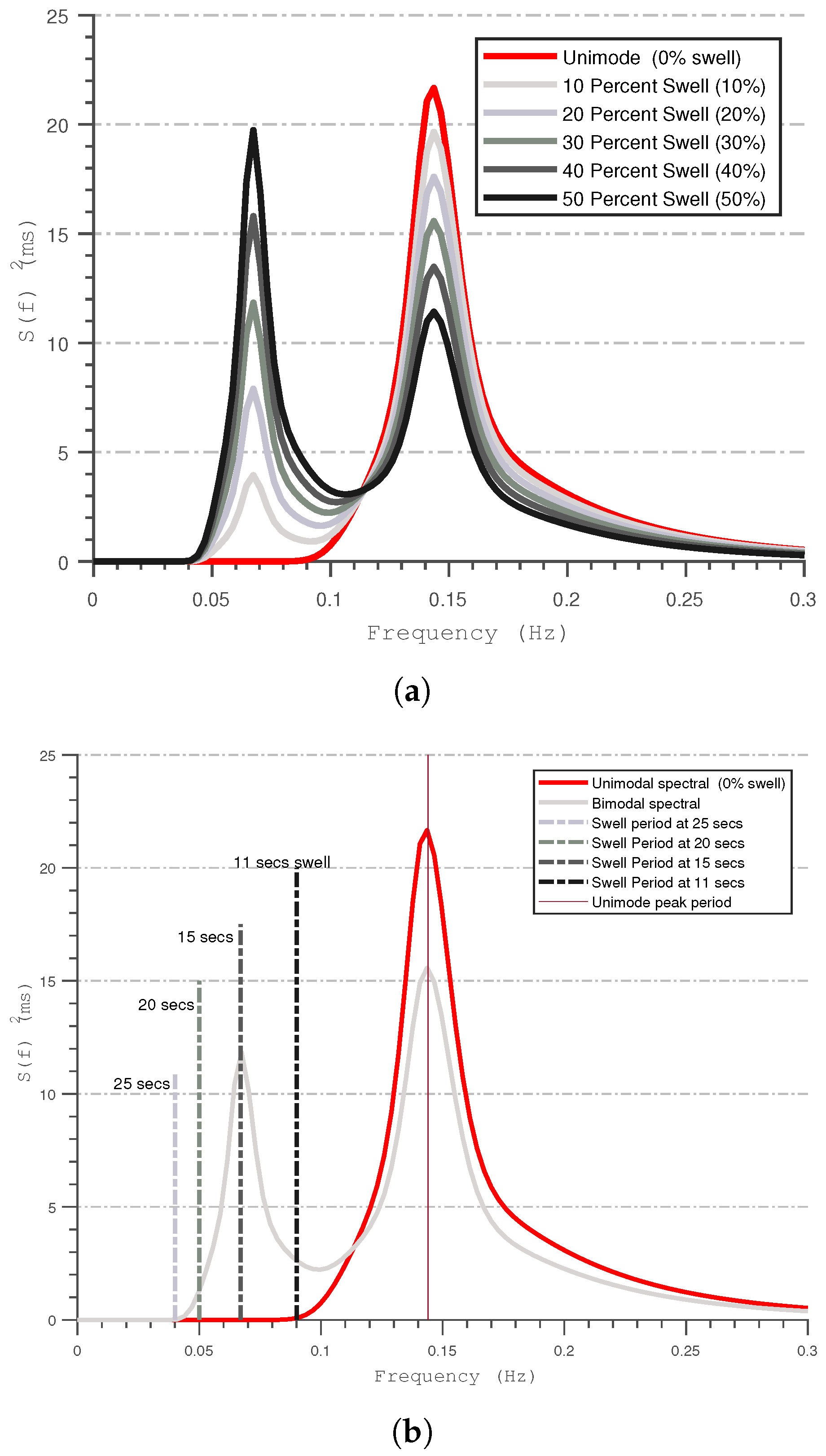
Figure 3 presents an example of a sea state with of 4 m and = 7 s. The swell component was fixed at a period varied from 11 s to 25 s while maintaining the same . Assuming an introduction of a 25 percent swell component into the sea, the remaining 75 percent of the energy will be allocated to the wind-sea using the SSER approach proposed by Guedes Soares [4] as stated in Equation (3). The exception to the rule here is that the analytical relationship was solved iteratively until the total energy in the system was conserved. This method gives a different definition of swell compared to that based on separation of frequency because the overlap between the swell and the wind waves was preserved in this method.
2.3. Ensuring Energy Conservation in the Bimodal Spectrum
As proposed in the previous section, the influence of swell presence in a sea state condition can be best examined with bimodal sea states when the overall energy in the sea can be conserved by both components of the wind and the swell present in the sea. This was achieved in this case by solving Equations (1)–(4) iteratively as illustrated in Figure 1. The resulting bimodal spectrum yields the same total energy given by Equation (4). As shown in Figure 3b, the newly computed significant wave height of the bimodal spectrum was ensured to be consistent with any swell percentage and swell frequency introduced. To achieve this condition, the entire Equations (1)–(4) were solved iteratively until the energy obtained for the significant wave height in Equation (5) is fulfilled in step 3 of Figure 1. The resulting bimodal spectrum was converted into time series using the Inverse Fast Fourier Transform IFFT technique.
2.4. Determination of Kurtosis and Skewness of the Bimodal Spectrum
The relationship between the kurtosis and the skewness of the energy conserved bimodal seas was examined using the method proposed by Marthinsen and Winterstein [20]. A second-order approximation of the resulting bimodal spectrum is determined using Equation (6). Moreover, different orders of spectrum moments are computed from order 1 to 4 designated as , , , and using the approaches detailed in Cavannie et al. [21].
The kurtosis, , can be computed using and , and is defined as,
1st, 2nd, 3rd and 4th moments can be computed as:
where skewness,
where and represent the sum and the difference of frequency effects observed from individual spectra combined.
2.5. Wave Height Extraction Using Numerical Model
To extract values of wave height for the assessment of the non-linearity characteristics of bimodal seas, a long numerical flume is necessary. The wave propagation model used for the present study is the validated IH2VOF by the IHC Cantabria Lara et al., ([22]). The numerical model is based on the Volume of Fluid (VOF) technique to solve the 2DV Reynolds Averaged Navier–Stokes (RANS) equations with turbulence transport functionalities and active wave absorption accurately implemented. IH2VOF model has been validated against several hydrodynamic scenarios including plane beaches and rubble mound breakwaters (see Lara et al., and Ruju et al. [22,23] for details).
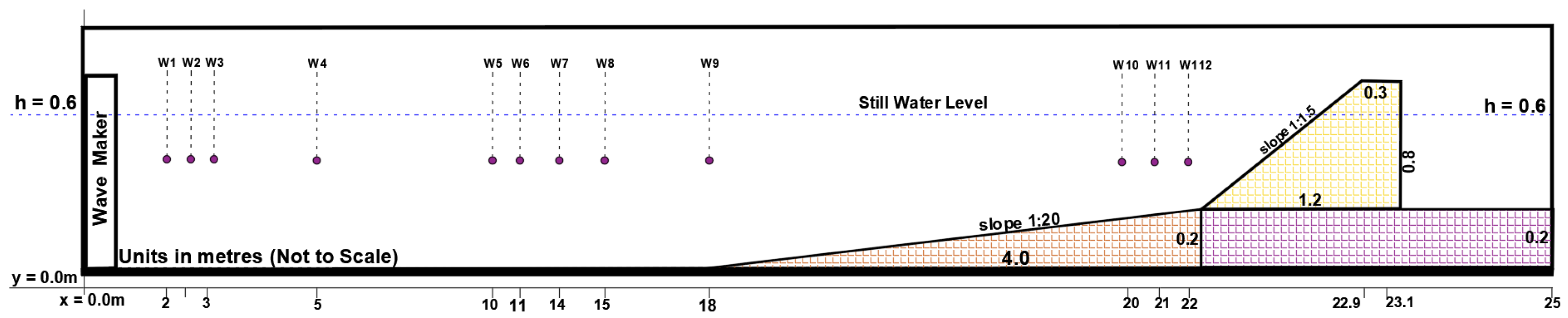
Surface elevations (time series) obtained from the inverse FFT were used to create sets of mesh-dependent pre-designed horizontal and vertical velocities based on the linear wave theory was used to drive the model. The computational domain discretised into 0.005 m on x-axes (33,514 meshes) and 0.01 m along y-axes mesh-sizes (51 meshes) were used to run the simulation with a time step of 0.004 s to maintain a stable simulation over a storm duration. As shown in Figure 4, wave gauges placed near both the wave-maker (W1, W2 and W3) and near the structures (W10, W11, and W12) were used to obtain the time series of the surface elevation. First three wave gauges are placed at 2 to 3 m from the wave maker while the last three are positioned near the structure within 20 to 22 m away from the wave maker.
The wave conditions tested in this study were presented in Table 1. The same grid sizes were applied in each case. Varying percentages of swell waves were introduced into the wind sea states and at different swell periods. The bimodal spectrum formed in this process were then converted into surface elevations which are used to drive the IH2VOF model as detailed in Section 2 above.
3. Results and Discussions
3.1. Analysis of Free Surface From the Energy-Conserved Bimodal Spectrum
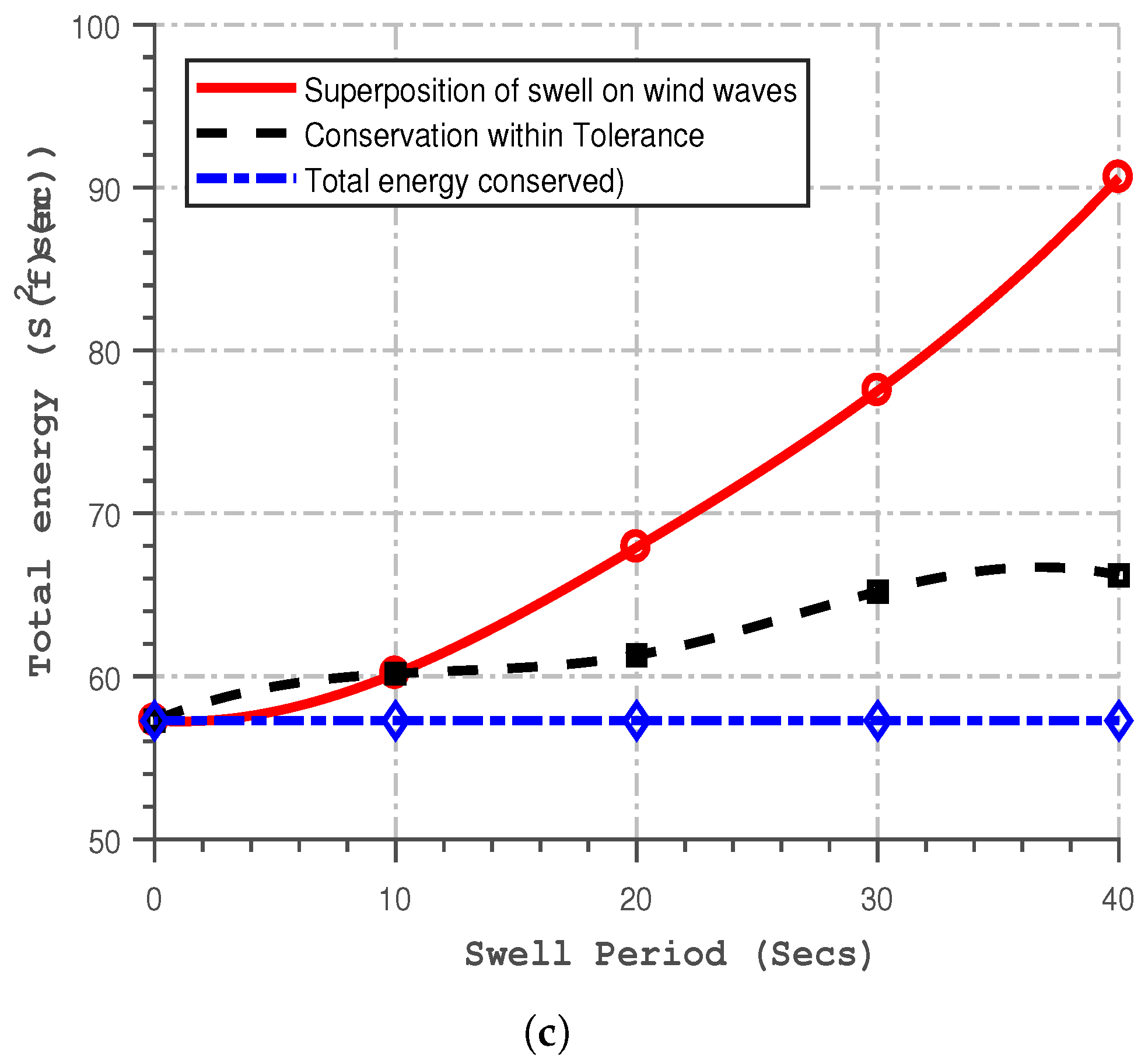
Examples of free surface derived from bimodal spectra are presented in Figure 5. The bimodal sea time series contained different swell percentages and the swell peak periods that were gradually varied as detailed in Table 1. As shown in Figure 5a,b, there is no significant graphical noticeable differences between the wave elevations of waves time series generated by different swell percentages. This could happen because the overall energy contained in the sea states are preserved even though different randomness was applied when obtaining the time series as presented in Figure 5c. Energy conservation was evident in Figure 5b by further inspection of the minimum and maximum values of the surface elevations. The values are fluctuating around a specific mean of minimum and maximum values of −0.1 m and 0.1 m respectively for the sea state (4 m, 7 s) investigated at a scale of 1:20. These results follow the standard weakly stationarity and ergodic assumptions of a sea state with zero mean described in Rychlik [24].
3.2. Analysis of Kurtosis and Skewness
Figure 6a–c presented the relationship between the auto-covariance function, ACF, with increasing overall swell percentages and swell periods of the individual wave characteristics extracted from the computational model. The cross-correlation function in Figure 6a reveals that by increasing the swell percentages of a sea state, the individual waves are still largely independent of each other. There is a slight decrease in the independence as the swell percentages increase from 25 to 75 percent swell sea conditions. This effect is similar to what is observed as the swell peak period increased from 11 s to 25 s in Figure 6b. Figure 6c presented the performance of skewness parameter with varying proportions of swell periods. As clearly shown in this figure, there is an inverse relationship. Skewness reduces with increasing swell peak periods. Skewness behaviour was tending towards a constant value as swell peak periods increases in the same sea state. Skewness behaviour was highest for the unimodal sea than for equivalent bimodal sea conditions. Also, reduction of skewness was observed with increasing swell percentages.
In total, as shown in Figure 6d, under the conserved energy bimodal sea states, there is a dynamic reduction in the relationship between the kurtosis and skewness as the swell percentage and the peak period increases. This is an increasing smooth and continuous exponential relationship that can be expressed as:
A sea state with 25 percent swell at a peak period of 11 s has the largest skewness-kurtosis relationship as compared with the lowest affinity relationship portrayed by the 75 percent swell at a much lower frequency of 25 s. The coefficient of kurtosis deviates significantly from linear predictions. The results obtained here near the structure are similar to those Forristall [3] observed on a shoaling beach.
4. Influence of Swell on Wave Height Distribution
4.1. Influence of Swell Period
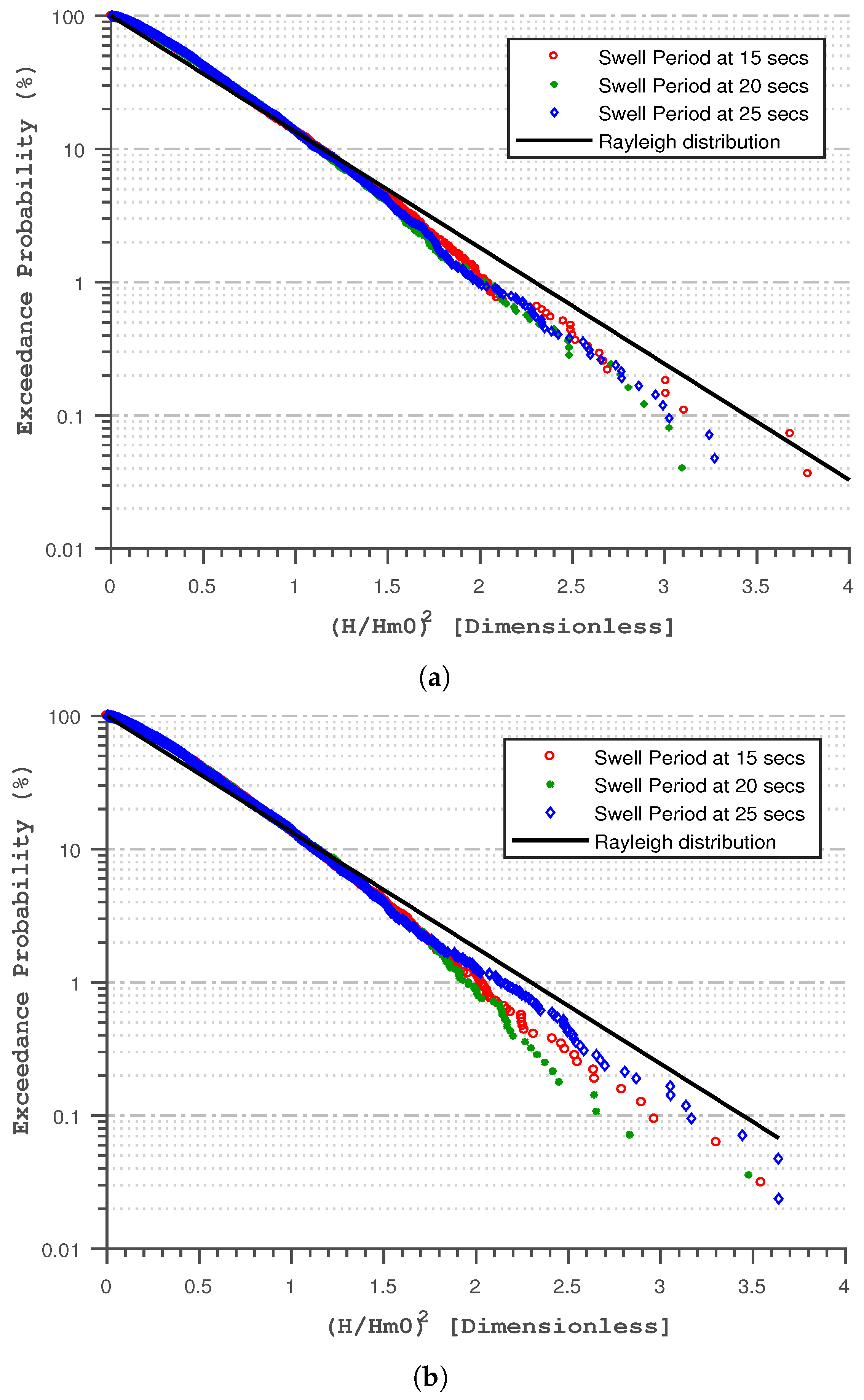
The probability distribution curves in Figure 7 show how wave height distribution is influenced by different frequencies of swell in the bimodal energy spectrum as observed both near and away from the structure.
If the waves followed a Rayleigh distribution, all the points would fall on the full straight line shown in each figure. Wave height distribution is greatly affected by the peak period of the swell. Non-linearity patterns are indicated by deviation from the Rayleigh linear scale, and strongly related to the swell peak period. This is because the Rayleigh distribution better represents narrow-band sea states such as observed by Toffoli and Monbaliu [25]. These deviations increase with the closeness of the two peak frequencies (for swell and wind) on the energy spectrum. Increasing the swell peak period in the energy spectrum expands the width occupied by the bimodal spectrum. This occurrence would in turn increased the overall spectra period obtainable from the resulting spectrum when transformed. In general, higher wave values deviates significantly from Rayleigh predictions. Boccotti [14] suggests that the waves become more unstable because of the non-linearities from long crested conditions. Further observations are that the non-linearities of wave height became more pronounced near the structure because of wave-wave interactions and through shoaling as they propagate into shallow waters.
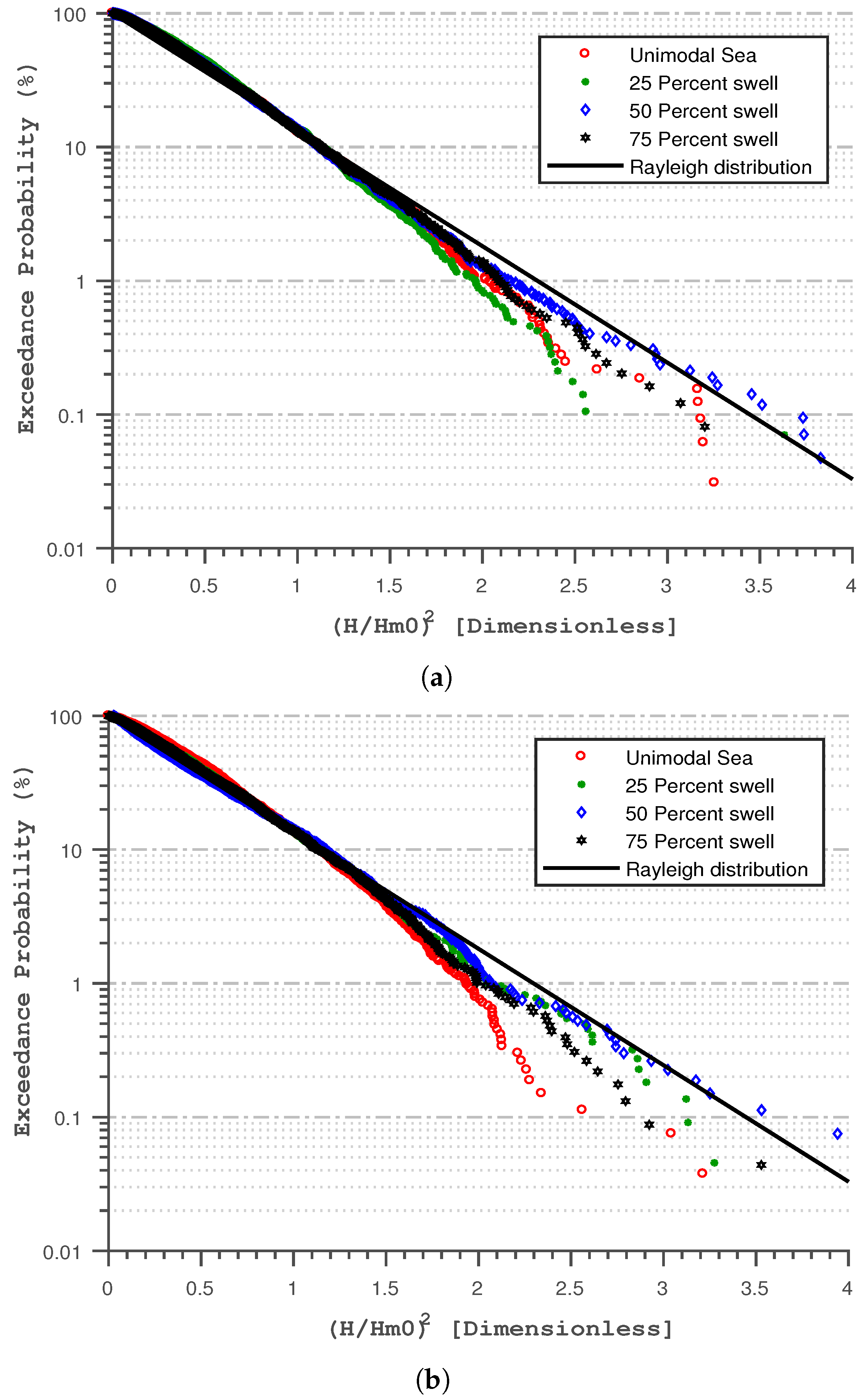
4.2. Influence of Swell Percentages
Following the previous section, Figure 8 depicts the wave height statistics within the domain for different swell percentages introduced into an energy-conserved sea state. The non-linearity patterns were extended to a unimodal sea. In all the sea cases considered (unimodal and bimodal), the non-linearity pattern was highest near the seawall than near the wave maker. This is expected because of the shoaling process and reflection created by the wave interaction with the sea wall. As shown in Figure 8, non-linearity behaviour is higher in the unimodal seas state than for the bimodal seas (in this case). This trend of non-linearities reduces with increasing swell percentages. However, some deviations from this trend are obssrved in 50 percent swell. This may be due to the uneven distribution of energy formed by the double jonswap spectra and may require further study.
4.3. Patterns of Wave Height Distribution
Figure 9a–f shows Weibull and the Rayleigh plots depicting the wave height distribution performance of different swell percentages in the bimodal sea states. In all the cases considered (both near and away the structure), wave height is better predicted by the Weibull distribution than the Rayleigh plots. However, both distributions show great agreement at representing lower to middle part of wave height values. Earlier deviations from normal were evident for Rayleigh distributions than for Weibull plot.
This trend gradually reduced as we approach the structure Figure 9b,d,e because more non-linearity patterns are possible by waves transformation caused by the wave-structure interactions. Also as expected, Rayleigh distribution underpredict higher waveheight values while the Weibull plots are over-predicting in a way. As observed in all cases, non-linear trends are greatest in the 25 percent swell in Figure 9b and was gradually reducing as the swell percentages increasing towards the 75 percent swell in Figure 9e,f. The observed behaviour is similar to the Petrova and Guedes Soares [26], wherein the non-linearities in the wave height distribution was also decreasing with increasing swell percentages in the bimodal sea provided there is a great identicality in their initial spectra where they are formed.
5. Conclusions
This paper has addressed the influence of swell in a bimodal sea states with constant energy content while varying swell peak periods and percentages. Specified bimodal spectra were converted into time series using inverse FFT. The time series was used to drive the VOF-model in a numerical domain. The downcrossing analyses of numerical wave-gauge results sampled from near the wavemaker and the structure were used to assess the physical non-linearity of the bimodal sea state. There is an increasing smooth and continuous exponential relationship between the skewness and kurtosis as the swell percentage and the peak period grows in an energy conserved bimodal sea. The extracted waveheight distribution on the Weibull and Rayleigh distribution plots to inspect the non-linearity imposed by wave-wave interactions and through dispersions as they propagate into shallow waters near the structure. The Weibull distributions produced the best fitness for wave patterns of high swell percentages considered. As the swell frequency and percentages in a bimodal sea, the relationship between the skewness and the kurtosis are tending towards a unimodal sea. The distribution of the waveheight on the Rayleigh model shows that the non-linearity increases with the distance away from the wave maker. This could be caused by the development of other physical processes like reflection, wave breaking, and other shoaling processes arising from wave-structure structure. In agreement with previous studies, the unimodal sea states showed the greatest non-linear bahavior however, non-linearity patterns vary as the swell grows. The Rayleigh distribution could not properly represent bimodal seas with wider spectral width and also overpredicts waveheight at low exceedances in these conditions.
Author Contributions
S.O. conceived and wrote the paper draft. S.O. performed the numerical simulations. H.K. and D.E.R. contributed to the analysis and discussion of the results and also revised the paper.
Funding
This research was funded by The Petroleum Technology Trust Fund (PTDF), Nigeria (Grants No. OSS/PHD/842/16).
Acknowledgments
The author will like to acknowledge Javier Lara not only for providing the IH2VOF codes for simulations, but also for instructions on implementation.
Conflicts of Interest
The authors declare no conflict of interest.
Abbreviations
The following abbreviations are used in this manuscript:
| ACF | Auto-covariance function |
| FFT | Fast Fourier Transform |
| IHC | The Environmental Hydraulics Institute Cantabria |
| IFFT | Inverse Fast Fourier Transform |
| H | Significant wave height |
| Jonswap | Joint North Sea Wave Project |
| RANS | Reynolds-Averaged Navier Stokes (RANS) |
| Kurtosis | |
| Skewness | |
| SSER | Sea-Swell energy ratio |
| UKCP | United kingdom climate projections |
| VOF | Volume of Fluid |
References
- Jenkins, G.; Murphy, J.; Sexton, D.; Lowe, J.; Jones, P.; Kilsby, C. UK Climate Projections: Briefing Report; Technical Report; Met Office Hadley Centre: Exeter, UK, 2009.
- Hawkes, P.J.; Coates, T.; Jones, R.J. Impacts of Bimodal Seas on Beaches, Hydraulic Research Wallingford; HR Wallingford Report; HR wallingford Lld.: Wallingford, UK, 1998; p. 80. [Google Scholar]
- Forristall, G. On the Statistical Distribution of Wave Heights in a Storm. Geophys. Res. 1978, 83, 2353–2358. [Google Scholar] [CrossRef]
- Guedes Soares, C. Representation of Double-Peaked Sea Wave Spectra. Ocean Eng. 1984, 11, 185–207. [Google Scholar] [CrossRef]
- Tayfun, A.; Fedele, F. Wave-height distributions and nonlinear effects. Ocean Eng. 2007, 34, 1631–1649. [Google Scholar] [CrossRef]
- Arena, F.; Guedes Soares, C. Nonlinear High Wave Groups in Bimodal Sea States. J. Waterw. Port Coast. Ocean Eng. 2009, 135, 69–79. [Google Scholar] [CrossRef]
- Burcharth, H.F. The effect of wave grouping on on-shore structures. Coast. Eng. 1978, 2, 189–199. [Google Scholar] [CrossRef] [Green Version]
- Battjes, J.A.; Groenendijk, H.W. Wave height distributions on shallow foreshores. Coast. Eng. 2000, 40, 161–182. [Google Scholar] [CrossRef]
- Reeve, D.; Chadwick, A.; Fleming, C. Coastal Engineering: Processes, Theory and Design Practice; Spon: London, UK, 2015; 518p. [Google Scholar]
- Longuet-Higgins, M.S. On the statistical distribution of the heights of sea waves. J. Mar. Res. 1952, 11. [Google Scholar] [CrossRef]
- Tayfun, M.A. Distribution of crest-to-trough waveheights. J. Waterw. Ports Coast. 1981, 116, 149–158. [Google Scholar]
- Naess, A. On the distribution of crest-to-trough waveheights. Ocean Eng. 1985, 12, 221–234. [Google Scholar] [CrossRef]
- Vinje, T. The statistical distribution of waveheights in a random seaway. Appl. Ocean Res. 1989, 11, 143–152. [Google Scholar] [CrossRef]
- Boccotti, P. Wave Mechanics for Ocean Engineering; Elsevier Science B.V.: Amsterdam, The Netherlands, 2000; p. 479. [Google Scholar]
- Rodriguez, G.; Guedes Soares, C.; Pacheco, M.; Perez-Martell, E. Wave Height Distribution in Mixed Sea States. Offshore Mech. Arct. Eng. 2002, 124, 34–40. [Google Scholar] [CrossRef]
- Petrova, P.G.; Guedes Soares, C. Wave height distributions in bimodal sea states from offshore basin. Ocean Eng. 2011, 38, 658–672. [Google Scholar] [CrossRef]
- Nørgaard, J.Q.H.; Lykke Andersen, T. Can the Rayleigh distribution be used to determine extreme wave heights in non-breaking swell conditions? Coast. Eng. 2016, 111, 50–59. [Google Scholar] [CrossRef]
- Hasselmann, K.; Barnett, T.; Bouws, E.; Carlson, H.; Cartwright, D.; Enke, K.; Ewing, J.; Gienapp, H.; Hasselmann, D.; Kruseman, P.; et al. Measurements of Wind-Wave Growth and Swell Decay during the Joint North Sea Wave Project (JONSWAP); Deutsches Hydrographisches Institut: Hamburg, Germany, 1973; Volume A8. [Google Scholar]
- Goda, Y. Random Seas and Design of Maritime Structures; World Scientific Publishing Co. Pte. Ltd.: Singapore, 2010; p. 708. [Google Scholar]
- Marthinsen, T.; Winterstein, S. On the skewness of random surface waves. In Proceedings of the 2nd International Offshore and Polar Engineering Conference, San Francisco, CA, USA, 14–19 June 1992; pp. 472–478. [Google Scholar]
- Cavannie, A.; Arhan, M.; Ezraty, R. A statistical relationship between individual heights and periods of storm waves. In Proceedings of the 1st Conference on Behaviour of Offshore Structures, Trondheim, Norway, 2–5 August 1976; pp. 354–360. [Google Scholar]
- Lara, J.L.; Ruju, A.; Losada, I. RANS modelling of long waves induced by a transient wave group on a beach. Proc. R. Soc. A 2011, 467, 1212–1242. [Google Scholar] [CrossRef]
- Ruju, A.; Lara, J.L.; Losada, I.J. Numerical analysis of run-up oscillations under dissipative conditions. Coast. Eng. 2014, 86, 45–56. [Google Scholar] [CrossRef]
- Rychlik, I.; Johannesson, P.; Leadbutter, M. Modelling and Statistical Analysis of Ocean-wave Data Using Transformed Gaussian Processes. Mar. Struct. 1997, 10, 13–47. [Google Scholar] [CrossRef]
- Toffoli, A.; Onorato, M.; Monbaliu, J. Wave statistics in unimodal and bimodal seas from a second-order model. Eur. J. Mech. B/Fluids 2006, 25, 649–661. [Google Scholar] [CrossRef]
- Petrova, P.G.; Guedes Soares, C. Distributions of nonlinear wave amplitudes and heights from laboratory generated following and crossing bimodal seas. Nat. Hazards Earth Syst. Sci. 2014, 14, 1207–1222. [Google Scholar] [CrossRef] [Green Version]
Figure 1.
Flow chart on the generation of an energy conserved bimodal spectrum.

Figure 2.
Building up of energy-conserved bimodal spectrum from separate swell and wind components. (a) Swell wave spectrum from Equation (2) for j; (b) Wind wave spectrum from Equation (2) for i; (c) Bimodal wave spectrum from wind and swell.

Figure 3.
An example of the development of energy-conserved bimodal spectrum. (a) Tested bimodal spectrum; (b) An energy-conserved bimodal showing different frequencies of swell; (c) Sample surface elevation obtained by Inverse Fast Fourier Transform (FFT).
Figure 3.
An example of the development of energy-conserved bimodal spectrum. (a) Tested bimodal spectrum; (b) An energy-conserved bimodal showing different frequencies of swell; (c) Sample surface elevation obtained by Inverse Fast Fourier Transform (FFT).


Figure 4.
Layout of a 2-D numerical model (not to scale) for a waveheight extraction using the wave gauges near the wavemaker and the structure.
Figure 4.
Layout of a 2-D numerical model (not to scale) for a waveheight extraction using the wave gauges near the wavemaker and the structure.

Figure 5.
Comparison of the different free surface elevations for different swell percentages at swell peak period of 25 s. (a) Free surface elevation obtained for different swell percentages as shown; (b) Analysis of the surface elevation shown in (a) above; (c) Comparison of total energy obtained for different methods of combining swell and wind.


Figure 6.
Time variance analysis of the effects swell periods and percentages in a bimodal sea with and . (a) Relationship between the Auto-covariance function ACF with increasing overall swell percentages in a bimodal sea; (b) Relationship between the ACF with increasing swell periods in a bimodal sea; (c) Variation of skewness with swell periods; (d) Variations of kurtosis against skewness for different swell periods.

Figure 7.
Effects of swell periods on wave height distribution near and away from the structure. (a) Wave height distribution for different swell periods observed away from the structure; (b) Distribution of wave height for different swell periods observed near the structure.
Figure 7.
Effects of swell periods on wave height distribution near and away from the structure. (a) Wave height distribution for different swell periods observed away from the structure; (b) Distribution of wave height for different swell periods observed near the structure.

Figure 8.
Effects of wave bi-modality caused by different swell percentages. (a) Wave height distribution for different swell percentages observed near the structure; (b) Distribution of wave heights for different swell percentages observed near the wave-maker.
Figure 8.
Effects of wave bi-modality caused by different swell percentages. (a) Wave height distribution for different swell percentages observed near the structure; (b) Distribution of wave heights for different swell percentages observed near the wave-maker.

Figure 9.
Comparisons of performance of wave height distribution using Weibull and Rayleigh plots for different swell percentages both away (a,c,e) and near the structure (b,d,f).
Figure 9.
Comparisons of performance of wave height distribution using Weibull and Rayleigh plots for different swell percentages both away (a,c,e) and near the structure (b,d,f).


Table 1.
Bimodal wave conditions tested in the present study.
| (m) | (s) | Swell Peak Periods (s) | Swell Percentages | Gamma |
|---|---|---|---|---|
| 1.0 | 7.0 | 15, 20, 25 | 25 | Wind = 3.3; Swell = 2.5 |
| 1.5 | 8.0 | 15, 20, 25 | 50 | Wind = 3.3; Swell = 2.5 |
| 2.0 | 9.0 | 15, 20, 25 | 75 | Wind = 3.3; Swell = 2.5 |
© 2019 by the authors. Licensee MDPI, Basel, Switzerland. This article is an open access article distributed under the terms and conditions of the Creative Commons Attribution (CC BY) license (http://creativecommons.org/licenses/by/4.0/).
Share and Cite
MDPI and ACS Style
Orimoloye, S.; Karunarathna, H.; Reeve, D.E. Effects of Swell on Wave Height Distribution of Energy-Conserved Bimodal Seas. J. Mar. Sci. Eng. 2019, 7, 79. https://doi.org/10.3390/jmse7030079
AMA Style
Orimoloye S, Karunarathna H, Reeve DE. Effects of Swell on Wave Height Distribution of Energy-Conserved Bimodal Seas. Journal of Marine Science and Engineering. 2019; 7(3):79. https://doi.org/10.3390/jmse7030079
Chicago/Turabian StyleOrimoloye, Stephen, Harshinie Karunarathna, and Dominic E. Reeve. 2019. "Effects of Swell on Wave Height Distribution of Energy-Conserved Bimodal Seas" Journal of Marine Science and Engineering 7, no. 3: 79. https://doi.org/10.3390/jmse7030079
Note that from the first issue of 2016, this journal uses article numbers instead of page numbers. See further details here.