Automatic Assessment of Individual Stem Shape Parameters in Forest Stands from TLS Point Clouds: Application in Pinus pinaster

Abstract

Tree morphological characteristics, particularly straightness and lean, significantly influence the value of the commercial products that can be obtained. Despite this, they are not usually evaluated in timber field inventories because traditional techniques are labor-intensive and largely subjective, hence the use of these parameters is limited to research and genetic breeding programs. Here, a non-destructive, fully automated methodology is presented that estimates the parameters for describing straightness and lean using terrestrial laser scanning (TLS) data. It is based on splitting stems into evenly spaced sections and estimating their centers, which are then used to automatically calculate the maximum sagitta, sinuosity, and lean of each tree. The methodology was applied in a breeding trial plot of Pinus pinaster, and the results obtained were compared with field measurements of straightness and lean based on visual classification. The methodology is robust to errors in the estimation of section centers, the basis for calculating shape parameters. Besides, its accuracy compares favorably with traditional field techniques, which often involve problems of misclassification. The new methodology is easy to use, less expensive, and overcomes the drawbacks of traditional field techniques for obtaining straightness and lean measurements. It can be modified to apply to any species and stand typology.

1. Introduction

Stem shape is a hugely relevant factor to consider in forestry, as it is closely related to wood quality and has a strong influence on sawmill performance, that is, on the percentage of profitable volume with respect to the volume of the log [1]. Consequently, it strongly conditions the use that can be made of a forest stand and its economic sustainability.

The term “stem shape” is usually used generically to refer to a wide range of characteristics, including straightness, conicity, tapering, lean, and even the presence of defects such as bracketing fork and prominences caused by the presence of knots. All these characteristics have great importance in forestry, but the specific importance of straightness and lean is widely recognized from both the scientific and technical perspective [2,3,4]. Stem straightness is particularly significant in forestry because it provides critical information for harvesting and sawing. Stems’ bucking optimization requires the very accurate determination of their shape to enable the cutting points along the stem to be established and to determine merchantable volumes according to particular specifications [5]. Furthermore, straightness is an important variable in trials, where selecting the straightest provenances is the basis for developing a tree breeding program [4]. In the case of lean, its importance was made clear in [6] and is based on the fact that it influences quality through increasing the proportion of reaction wood [7]; also it is, an expression of the adaptive growth of a tree [8] and a reaction to external loads (e.g., snowfall, stones…) that influences tree growth. Reaction wood (which forms in place of normal wood as a response to gravity meaning its cambial cells are oriented other than vertically) usually has a higher density. Although its mechanical properties are not reduced, it undergoes greater deformations during the drying processes and tends to break more easily; the reason being it is undesirable for wood processing purposes [9].

To measure the straightness of a stem the most commonly used parameter is sweep, which is traditionally defined as the maximum sagitta per meter of the stem [10]. However, sweep is not the only indicator of straightness; there are others such as sinuosity which are also of great interest. Sinuosity is expressed as the quotient between the line (not necessarily straight) which defines the axis of the stem and the Euclidean distance (straight line) between the end points of the stem [11]. As for the case of lean, it is defined as the angular deviation of a tree stem from a vertically upright position [12].

Fieldwork approaches to collecting data on such variables range from visual classifications made by one or more observers that group trees according to predefined categories, a very common methodology in tree breeding programs, to more evolved systems which use measurements (from calipers, measuring tapes and hypsometers) mainly based on the deviation or lean of the tree axis [10]. However, even with methods that use actual field measurements, results are still subject to observer´s interpretation, which is highly influenced by their experience and the criteria used, as well as by the characteristics of the stand. In the specific case of stem straightness, data on standing trees can also be obtained from localized or national stem curve models [5], but their wide scope of application makes them too imprecise to get accurate results at the individual tree level. Due to all the above, it is difficult to accurately measure complex stem shapes using conventional field investigation methods [2] which is why stem shape variables are not habitually measured as part of regular inventories [13]. This lack of measurements is especially notable in tree breeding programs of conifers in general (pines in particular) despite stem shape and branch angle assessment being very important [14,15]. In addition to these difficulties, and despite their relevance, in most cases it is not possible or practical to measure the variables implicated in straightness for every single tree in a plot using traditional fieldwork approaches since individual tree measurement is costly and labor intensive [16].

The use of remote sensing techniques, and more specifically the use of TLS (terrestrial laser scanning) can be very valuable in the estimation of stem shape. TLS acquires high resolution three-dimensional point clouds of the study area, which provides a reliable representation of the structure of the trees within the stands at the time when data were collected [17]. The fact that data are collected from the ground makes this technology especially suitable for studying stem profiles. In spite of this, there are only a few studies that have focused their efforts on the calculation of shape variables such as straightness and lean [9,18,19,20] or to the study of the presence and distribution of branches [21,22,23,24]. This may be explained by a combination of issues such as the high price of most scanning devices [25] and the lack of algorithms and software applications to calculate shape variables automatically [26] and which also requires expert knowledge to obtain reliable results. However, the general trend is slowly changing, equipment prices are gradually falling [27], and the proliferation of methodological developments which automatize data processing and analysis tasks is well under way [28,29,30]. Presumably, then, TLS will be a fundamental technology in forest inventories in the near future [31] and will make the automatic measurement of shape variables, such as straightness and lean, possible in regular inventories with minimal effort. For this to happen in a cost-effective and simple way, the automation of point cloud processing with readily available and easy-to-use software capable of extracting information related to important forest attributes is essential [1,26].

The aims of this study are two-fold: (i) To develop a methodology that allows the measurement of straightness (maximum sagitta and sinuosity) and lean automatically at the individual tree level from data captured with TLS; and (ii) to compare the results obtained with measurements made in the field by traditional methods (categorical visual classification that groups trees into classes).

2. Materials and Methods

2.1. Data Collection and Inventory

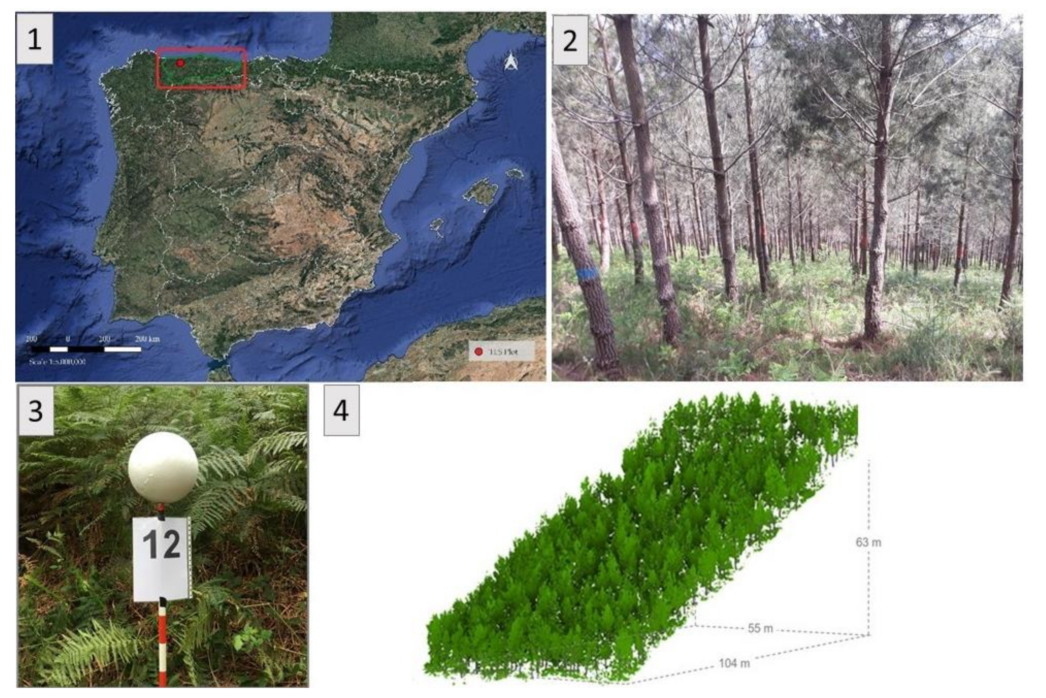
The study area is located in the autonomous region of Asturias (Northern Spain) (Figure 1(1)), characterized by an oceanic climate, with abundant rainfall throughout the year and mild temperatures in both winter and summer. The soils are siliceous. The plot where the study was carried out belongs to a network of trials for the National Tree Breeding program of Pinus pinaster, a species with a particular tendency to tortuosity. It has an approximate area of 5700 m². The terrain is irregular with high slope (>60%) (Figure 1(4)) and the presence of various shrub species such as Ulex, Ericas, and Pteridium, among others (Figure 1(2)). Both these characteristics contribute to making this study area a challenging one. It was planted in 2005 following an experimental design of four randomized blocks, where 225 families were planted, each family in a row of four trees. Some of the families are from the region of the plantation (Asturias) while others are from various places within Italy, France, Spain, Portugal, and the north of Africa. A genetic thinning (where also fallen trees were removed) was carried out in 2018 resulting in the current number of trees which is 408 (806 stems/ha).

Data acquisition was accomplished in November 2018 using a TLS FAROFocus3D. Twenty-four scanning paths were necessary to ensure full coverage and minimize the effect of occlusions. Polystyrene spheres of 25 cm diameter fixed to surveying rods were used to merge the point clouds of individual scans into a unified coordinate system (Figure 1(3)). Moreover, the position of the spheres was measured in the field using GNSS (Global Navigation Satellite System), thereby ensuring that the unified point cloud had absolute coordinates. The resulting point cloud had approximately 150 million points after removing redundant points within 6 mm (average density ~26,300 points/m²).

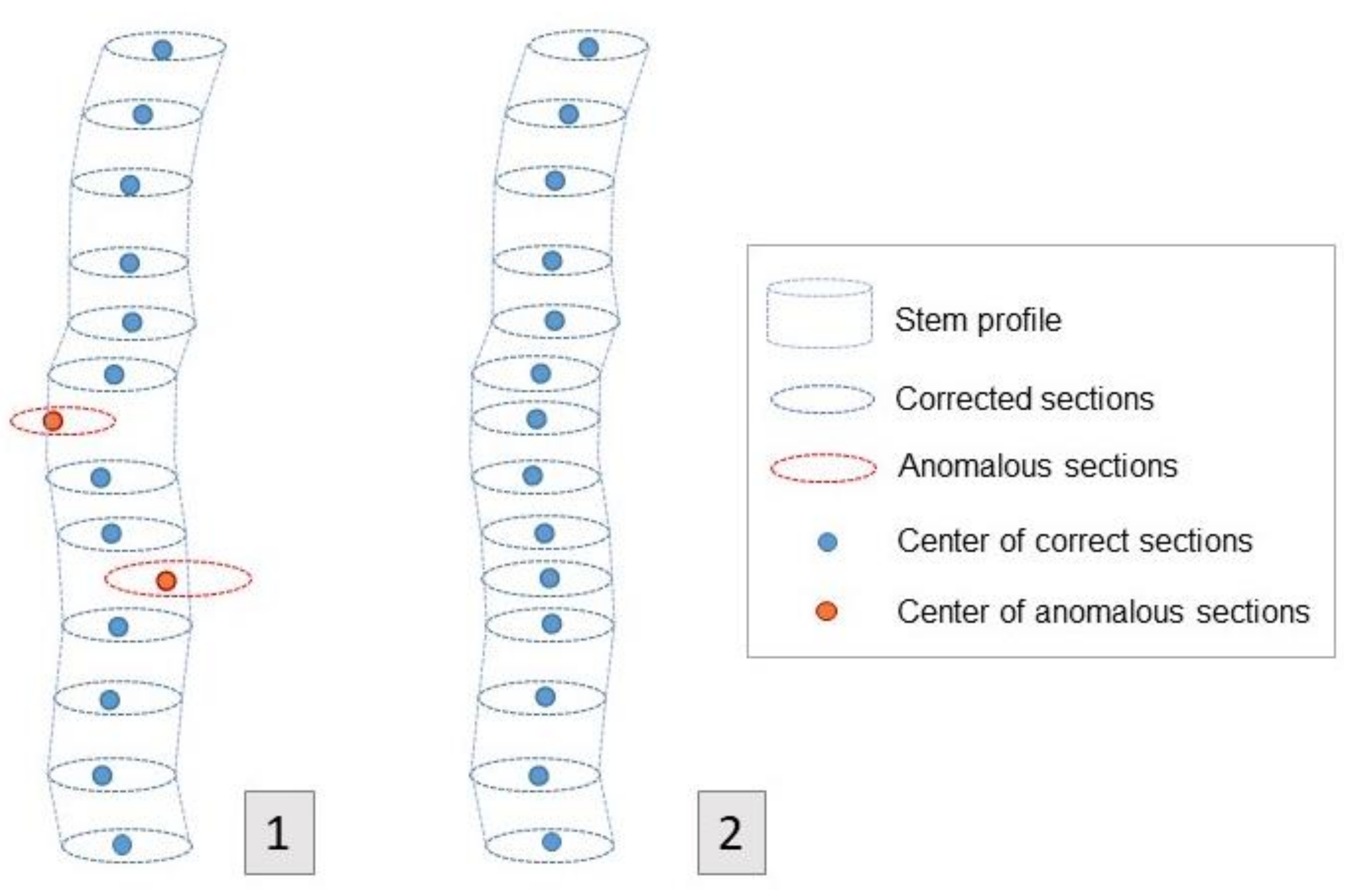
The point cloud (Figure 1(4)) was analyzed with the methodology for the automatic estimation of dbh and h described in [32,33]. As a result, for each tree, measurements of the diameters of the sections along the stem (spaced 20 cm apart, from 0.5 over the ground to 4.9 m) as well as their centers (defined by X, Y, Z coordinates) were automatically obtained (Figure 2(1)).

Some of the trees did not have the complete range of sections mainly due to (i) the number of points in a section being insufficient to perform the circle fitting or (ii) sections presented anomalies that the methodology detected automatically. In this regard, the methodology includes several filters to detect anomalies [32,33] so the potentially ‘wrong’ sections are flagged for revision by a human operator who checks whether the fitting is correct and/or if it is possible to fit the circle manually.

Moreover, as described in [33] to have a reference for the data calculated by the algorithm, diameter fitting was manually conducted in the point cloud twice for the same section, each time by a different operator (Op₁ and Op₂). As a result, the centers of the sections for all the individual trees within the plot were available and served two purposes: (i) as reference data to assess the performance of the algorithm and (ii) to correct those sections which were labeled as anomalous by the algorithm (Figure 2(1)) to ensure data used to estimate stem shape variables were free of outliers (Figure 2(2)). If a circle obtained and flagged by the algorithm was incorrect but there were enough points to visually estimate its size and position, the operator fitted the circle manually.

In parallel to TLS data acquisition, dbh was measured in the field with a caliper, to the nearest 1 mm, and h, to the nearest 10 cm, using a digital hypsometer (Vertex IV 360°). As a complement to this inventory data, all the tree stems within the plot were also geo-positioned using the same GNSS as used for the TLS spheres and a total station. This allowed the inventoried trees to be related to those in the point cloud, making comparisons between the two data sources possible. The average dbh and h for the plot were 17.6 cm and 10.20 m respectively.

Regarding conducting inventories of shape variables in the field (as mentioned in Section 1) in tree breeding programs, visual classifications that group the trees according to predefined categories have been widely used as selection criteria over the years to assess stem straightness and lean. In this study, these variables were visually assessed at an individual tree level by a field observer using the classification proposed by [2] for Pinus pinaster which is detailed in

Table 1. Scale of values used as a reference to measure stem shape variables in the field.

Category	Straightness	Lean
1	Straight	Lean not appreciable at first sight
2	Curved in the intermediate or basal zone and less than twice the dbh	Lean appreciable up to 15° (referred to the vertical)
3	Curved in the intermediate or basal zone and more than twice the dbh	Lean greater than 15° referred to the vertical)

.

In the next section the steps to be followed to estimate straightness and lean from the TLS point cloud are detailed.

2.2. Stem Shape Variables Estimation from TLS Data

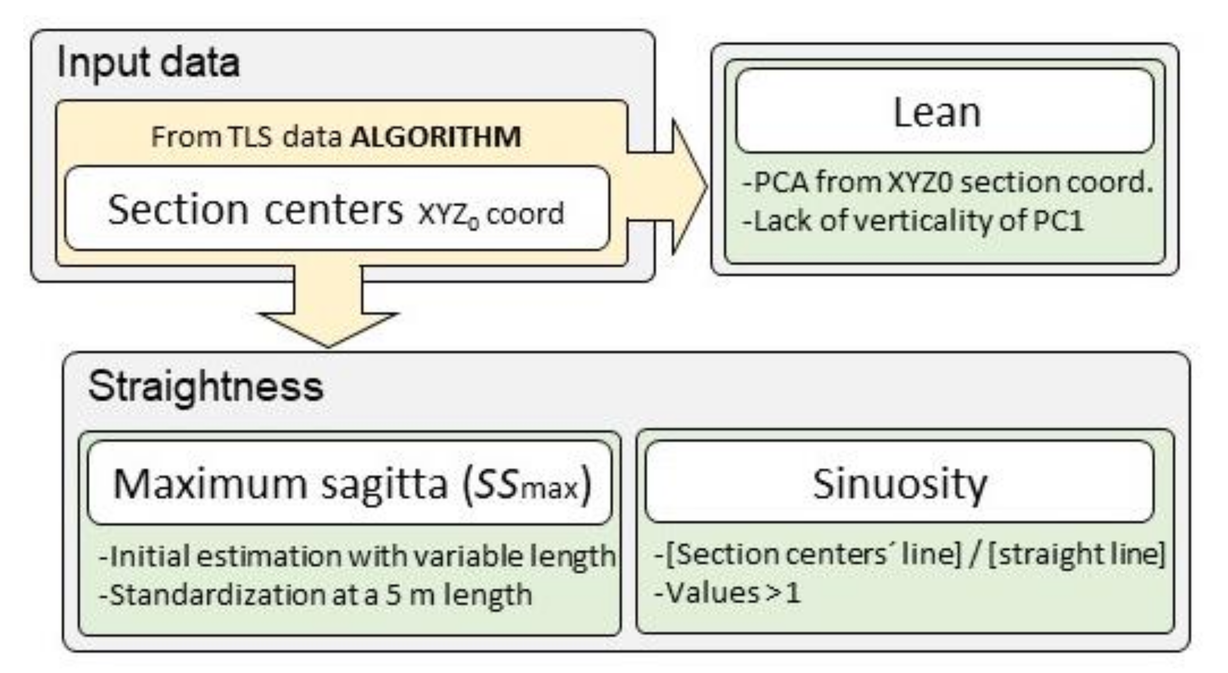
As shown in Figure 3, our method automatically calculates the lean angle and straightness parameters (maximum sagitta and sinuosity) from the exact location of the centers of the sections along the stems in a plot. The coordinates of all the sections available for each stem are used to define a polyline that allows the estimation of deviations from ideal straight and/or vertical stem axes.

The centers of the stem sections for each tree are the only input data necessary for straightness and lean estimations. Each coordinate (X, Y, and Z) is stored in an independent array with as many rows as trees in the plot, and as many columns as sections. The workflow for straightness and lean estimations has been implemented in a script written in Python, which enables these variables to be automatically obtained for each individual tree. Consequently, the methodology can be applied in datasets with different characteristics (e.g., species, stand conditions, slope) in a simple and fast way.

2.2.1. Straightness

For straightness assessment, the calculation of two variables, maximum sagitta and sinuosity, has been implemented in the methodology. The steps needed for their calculation are explained in detail below.

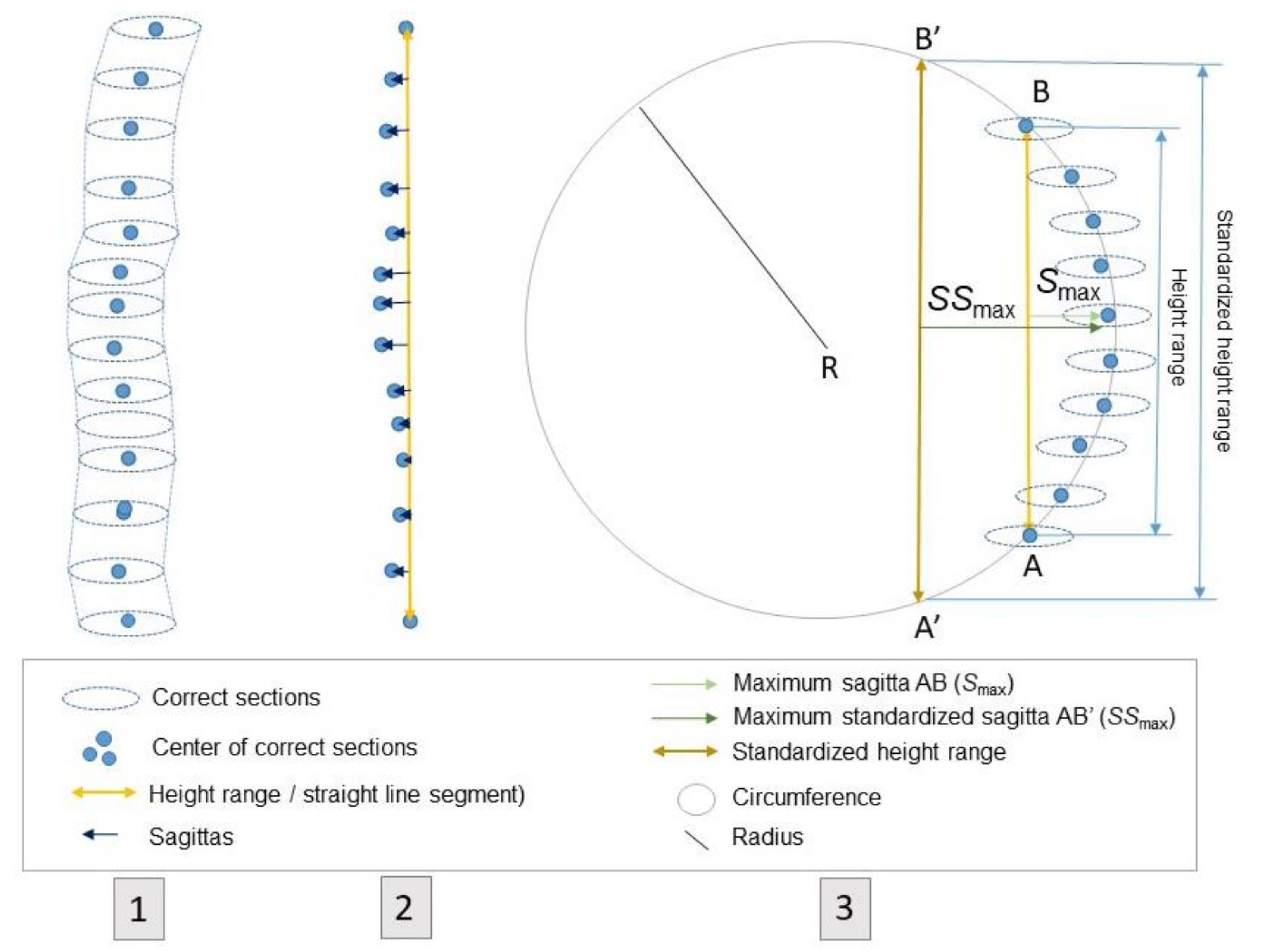
For each tree, the reference for the sagitta is taken from the straight line segment connecting the centers of the end sections. The sagitta of each section is then calculated as the distance between the center of the section (Figure 4(1)) and the straight line segment. The maximum sagitta (hereafter, S_max), as well as its position in the stem is identified (Figure 4(2)).

As explained in Section 2.1, some trees do not have data along the full height range (i.e., 23 sections over 4.4 m: from 0.5 to 4.9 m from the ground). In these cases, the sagitta is standardized to the highest height obtained for the dataset (hereafter, standardized height range, i.e., 4.4 m) so that the results obtained for each individual tree within the plot are comparable. To do this, the centers are considered to be distributed around a circumference of radius R (Figure 4(3)). R is calculated using the formula that relates the radius of a circumference with the sagitta of its arc and the length of the chord that connects the two ends of the arc. In this case, the sagitta is the S_max and the chord is the height range for each tree. From these two variables, R can be estimated as in Equation (2). Once the value of R is known for each tree, the maximum standardized sagitta (hereafter SS_max) can be obtained for the standardized height range, this time, by isolating the variable in Equation (1).

$$R=\frac{{\left[S_{max} AB\right]}^2+{\left[Height range/2\right]}^2}{2\ast {\left[S_{max} AB\right]}^{}}$$

(1)

The sinuosity of a line is calculated as the quotient between its length and the length of a reference line. In the case of a tree, that reference line is the straight line segment that joins the end points of the stem, and its length (L) is calculated as the sum of the rectilinear segments that connect the centers of the stem sections, as in Equation (2). According to this, the minimum value for sinuosity is 1, which means no sinuosity.

$$Sinuosity=\frac{L}{height range}$$

(2)

2.2.2. Lean

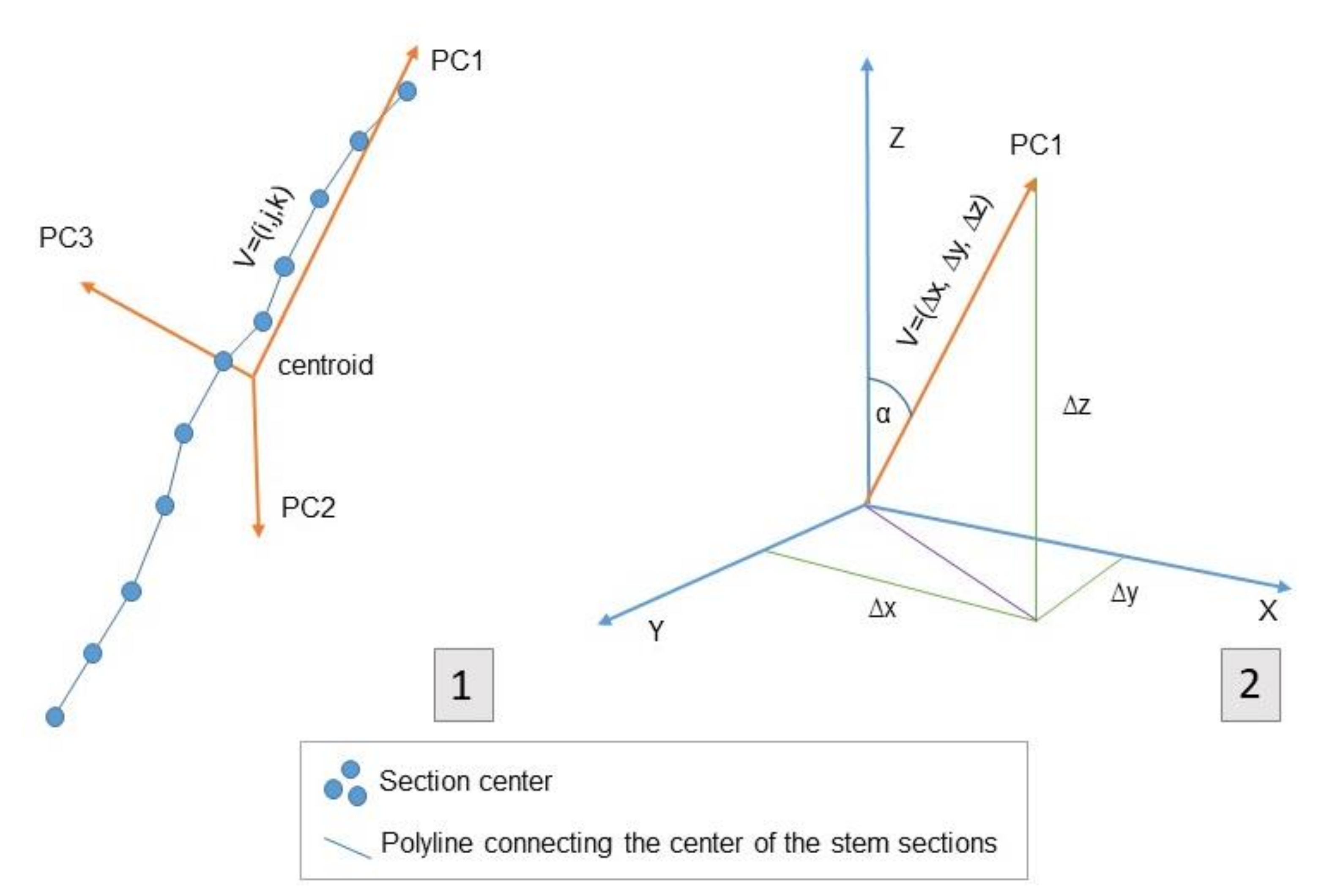
A principal component analysis (PCA) based on the X, Y, Z coordinates of section centers was carried out. When this type of analysis is applied to a tree-dimensional point cloud, three principal components (directions), which can be considered as three perpendicular coordinate axes, are created (PC1, PC2, and PC3) (Figure 5(1)). By definition, PC1 will follow the direction with the greatest variance possible. Since tree stems are eminently linear objects, the direction of the first component follows the direction of the tree axis, and from there, the lean, or lack of verticality, is calculated as in Equation (3) (Figure 5(2)).

$$\alpha =arctan\frac{\left|\Delta z\right|}{\sqrt{\Delta x^2+\Delta y^2}}$$

(3)

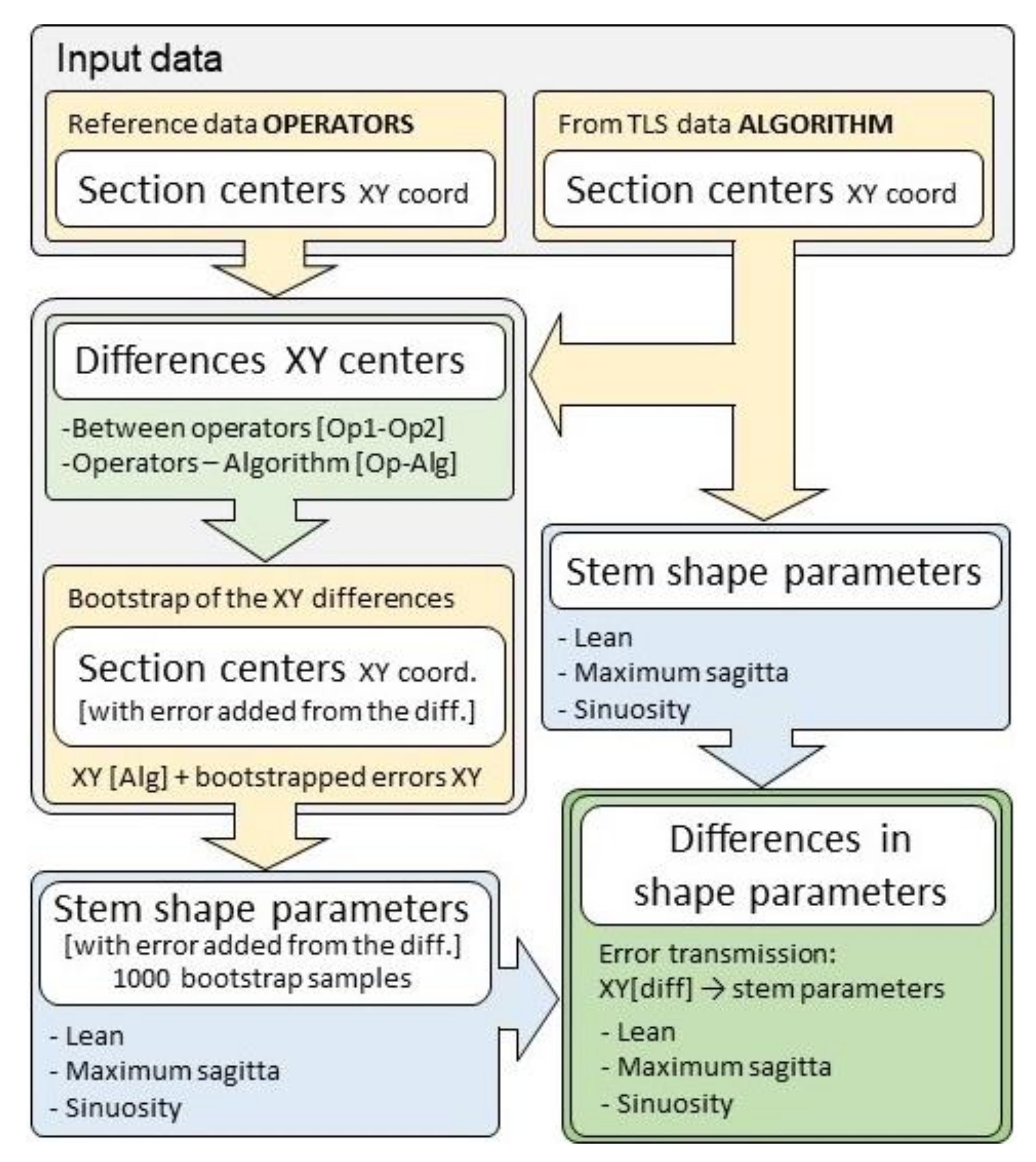
2.3. Validation Procedure

The only input data that the methodology uses to estimate the shape variables are the X, Y, Z coordinates of the centers of the sections, and errors will be transmitted to the same variables. Based on that, the methodology’s performance is assessed in terms of error propagation, from the position of the centers of the sections, to the maximum standardized sagitta, sinuosity, and lean. Manual measurements of the centers of the sections (X_op, Y_op) (see Section 2.1) have been considered as ground truth for the comparisons through the workflow explained in Figure 6. In this figure Op₁, Op₂ refer to manual measurements made by two different operators. Op refers to a random choice between diameters from Op₁ or from Op₂ that is used to minimize potential biases by either of the operators that might be imperceptible to the naked eye.

The differences between the two operators (Op₁-Op₂) and between the operators and the algorithm (Op-Alg) in positioning the sections’ centers were calculated. A bootstrap analysis was conducted to study the propagation of the errors from the center of the sections to maximum sagitta, lean, and sinuosity, considering that the distribution of these errors was not known. First, the initial values of these three variables were calculated for each tree given the coordinates (X, Y). Then, 1000 bootstraps samples of dimension N · M (N and M being the number of stems and number of sections, respectively) were constructed by resampling with replacement the initial values of the errors for each section. Then, the errors were obtained for each case and added to the initial X, Y coordinates of the centers estimated by the algorithm. With the new coordinates as a starting point, the maximum standardized sagitta, sinuosity, and lean of all the trees were recalculated. Finally, the results obtained were compared with the original estimates of the algorithm. From the differences between them, the density function of the differences was represented graphically, for each scenario and variable (distances between the centers of the sections, maximum standardized sagitta, sinuosity, and lean).

Regarding traditional estimations, comparing a continuous variable (from TLS data) and a categorical one (from a field inventory) is not straightforward due to their different natures. However, it is possible to evaluate if the categorization of the trees in the field as per their straightness and lean follows a similar pattern to that obtained with TLS. The procedure consists of grouping the trees on the plot following the traditional method (Table 1), and then calculating the two shape variables for each tree in each category using the TLS observations. Then, the probability density functions for each variable and for each category were compared. The comparison was done both visually and numerically. Numerical analysis was carried out by analyzing the statistics of both variables and through a Tukey-Kramer test [34,35] that compares the individual means from an analysis of variance of several samples with different characteristics.

3. Results

3.1. Stem Shape Variables from TLS

Once the methodology was tested in the plot, the shape variables were obtained for 385 of the initial 408 trees. The missing trees were either poorly defined in the point cloud or had a very small number of sections. In the first case, it was not possible to apply the methodology to them, while in the second case the results obtained were unreliable.

Table 2. Descriptive statistics of shape variables estimated from the TLS point cloud.

	Minimum	Maximum	Mean	Deviation	Median	Mode
Lean (°)	0.150	14.100	4.010	2.604	3.686	1.000
Maximum standardized sagitta (m)	0.020	0.390	0.104	0.058	0.092	0.094
Sinuosity (adimensional)	1.000	1.250	1.008	0.018	1.004	1.003

summarizes the minimum, maximum, mean, standard deviation, median, and mode of the shape variables estimated by the methodology.

The range of the lean values was low (14°); the maximum value corresponded to a tree classified as not leaning in the field. These results demonstrate that the trees were mostly slightly inclined. The standard deviation was around 0.5°, with lean values not widely dispersed around the mean. According to the median and mode values, the distribution had negative skew, and the range was small, which means that there was little variability in the lean values.

Regarding maximum standardized sagitta statistics, the trees in the plot can be considered as straight in most cases given their average value of 10.4 cm, which was very close to the average radius of the trees within the plot (8.8 cm). Standard deviation was approximately equivalent to half the mean value, and the distribution negatively skewed in terms of the median and mode values. The range was around 37 cm, indicating considerable variation in the maximum sagitta values. Regarding sinuosity, average values were close to 1 (no sinuosity), while the standard deviation was low, indicating an overall reduced stem tortuosity. The distribution shows negative skewness, and the range is small, which means that there was little variability in the sinuosity values. 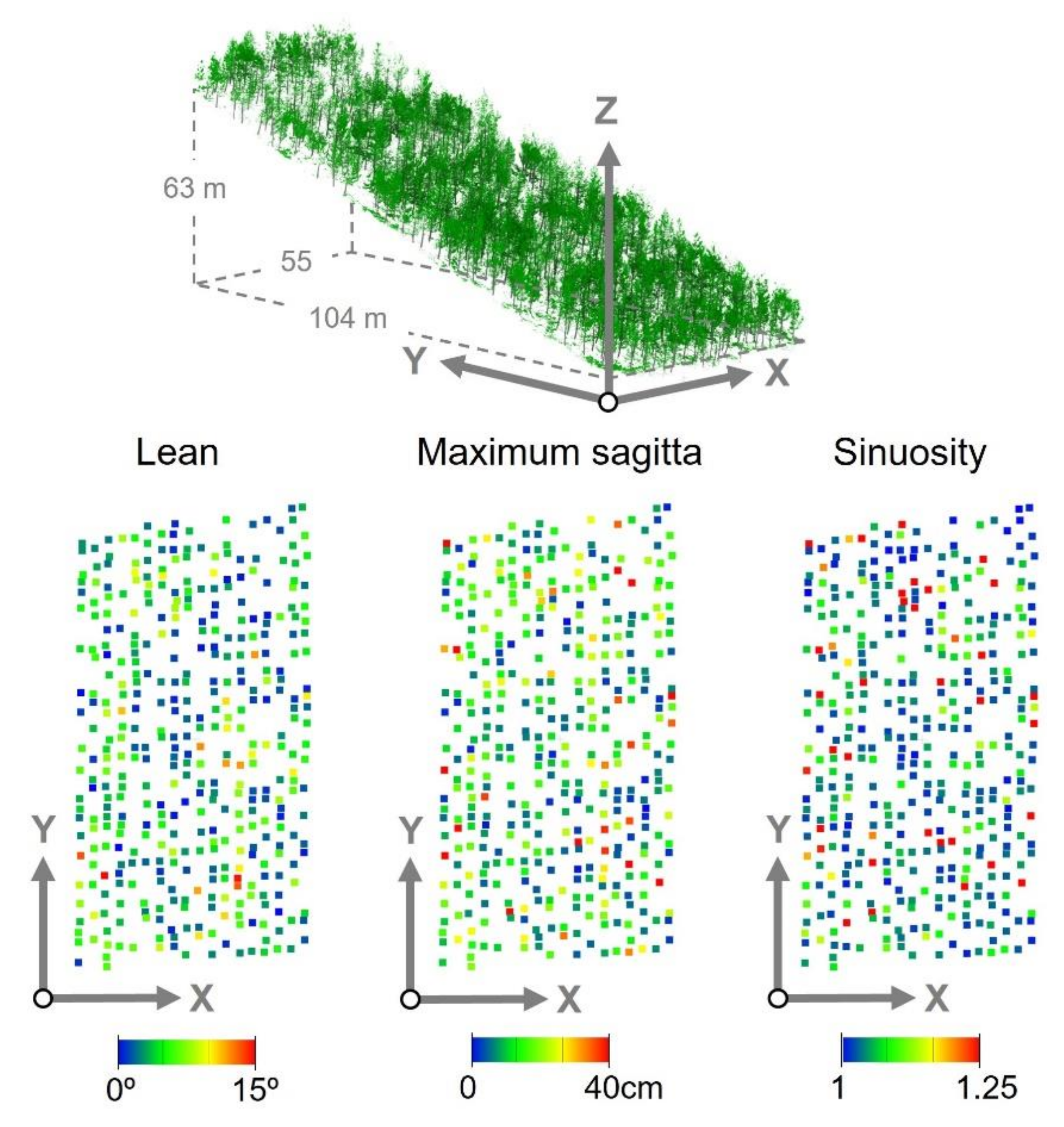Figure 7 shows the spatial distribution of the stem-shaped variables obtained in the study plot.

3.2. Validation Results

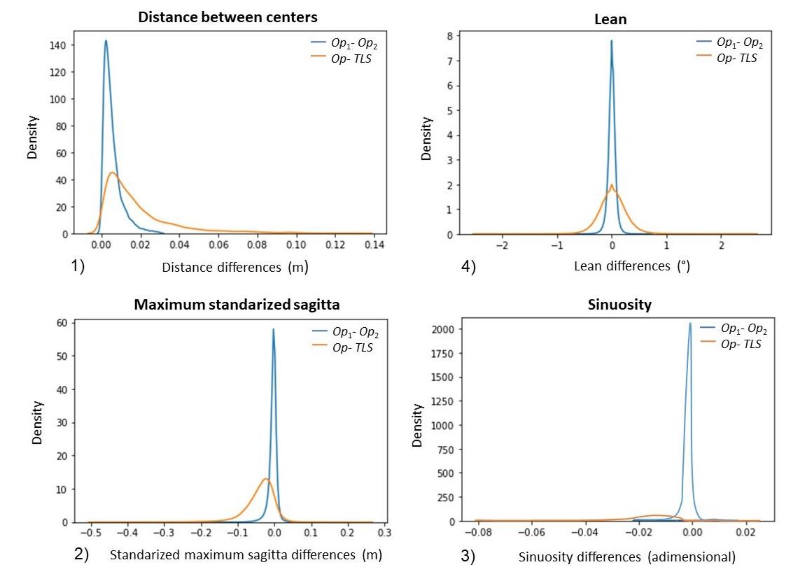
The results of assessing the methodology’s performance are shown in Figure 8. The probability density functions obtained as in the procedure explained in Section 2.3, were grouped according to the assessed variable and the comparison between operators (Op₁-Op₂) and operators-algorithm (Op-Alg).

Regarding the discrepancies between the centers of the sections (Figure 8(1)), the trend was similar in the two comparisons, with low values in general terms. As expected, the lowest values (less than 2% in 97% of the estimations) were obtained when comparing the estimations of the two operators. When the operator estimations were compared with the algorithm (Op-Alg), the discrepancies were slightly higher but still less than 4 cm in 90% of the estimates. The trend was similar for the results obtained for lean (Figure 8(4)) and maximum standardized sagitta (Figure 8(2)). For lean, discrepancies were extremely low when comparing Op₁ and Op₂, with less than 0.25° in 99% of the estimates. Regarding Op-Alg, the differences were a little higher, but they were still only between −0.5 and 0.5°, in 95% of the cases, so they were practically insignificant. The same occurred with the maximum standardized sagitta, where the lowest differences were computed for Op₁-Op_2, with 99% of differences in the estimates being below 5 cm. There was a slight bias in this case showing TLS tended to estimate bigger sagittas than the operators. The comparison between Op-Alg showed 92% of differences in the estimates to be below 10 cm. Finally, in the case of sinuosity (Figure 8(3)), differences between operators were practically negligible (very close to 0) on most occasions, while the differences between algorithm and operators were mostly around −0.015. The distribution was relatively uniform but still had a slight negative bias.

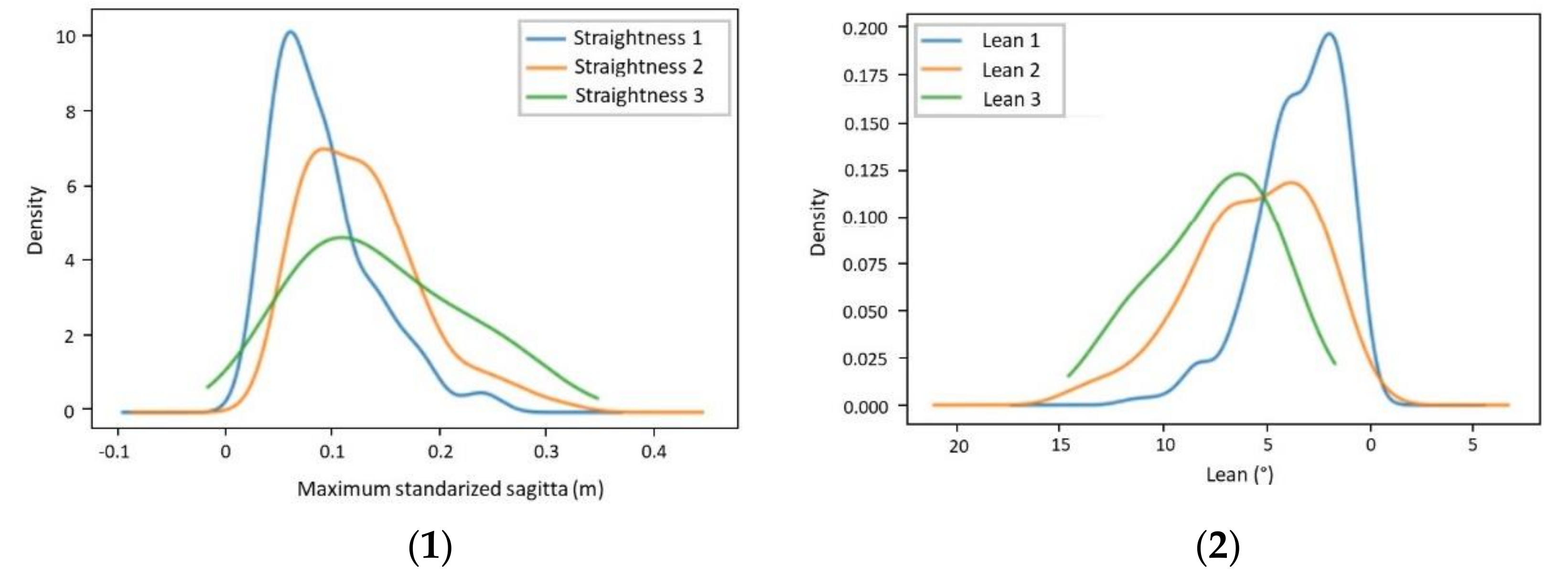
As for the comparison with traditional estimations, Figure 9 shows the probability density functions obtained for the trees within the study plot: one for each of the three categories under study established following the criteria in Table 1. Specifically, Figure 9(1) shows the three curves corresponding to the SS_max and Figure 9(2) shows those relative to the lean. In the case of the SS_max there was a high degree of overlap among the three categories, especially 2 and 3, which is an indicator that the boundaries between them were not well defined.

There was a tendency for SS_max to increase as category value increased. In category 1, most of the trees were around 5 cm, while in the other two categories, the peak of the density function was slightly shifted to the right, indicating a greater frequency of higher SS_max values. In the case of lean, the results were very similar. The curves show a high degree of overlap and reveal a slight decrease in the lean value as the category number increases. Moreover, it is observed that the peak of the distribution is very close to 0° in class 1 and slightly displaced to the left in classes 2 and 3.

Table 3. Maximum standardized sagitta (SS_max) and lean statistics obtained for the different categories shown in the probability density functions.

	Maximum Standardized Sagitta (m)					Lean (°)
	NS1	Mean	Deviation	Minimum	Maximum	NL1	Mean	Deviation	Minimum	Maximum
1	260	0.095	0.060	0.020	0.355	272	3.352	2.068	0.149	11.573
2	120	0.139	0.080	0.047	0.390	108	5.633	3.051	0.206	14.102
3	5	0.144	0.075	0.074	0.256	5	7.026	2.651	4.870	11.314

¹ N_S, N_L are the number of trees included in each category of straightness and lean respectively according to field inventory.

summarizes the descriptive statistics (mean, median, and standard deviation) of the maximum standardized sagitta and lean by category. In view of the results, the trend previously detected in the probability density functions is confirmed by the descriptive statistics. In the case of SS_max, mean values increase with the category number (see Table 1). Between categories 1 and 2 the increase is 4.4 cm, while between 2 and 3, it is only 0.5 cm.

In the case of lean, the situation also follows a clear trend: there is a decrease in its value as the field category number increases, which indicates that, in general terms, the trees are more inclined in the higher categories than in the first. The biggest increment in the mean value is between category 1 and 2 (2.28°), while between categories 2 and 3 it is only 1.39°.

Similar conclusions were obtained by performing a Tukey-Kramer test to compare the means between the three categories. For a significance level α = 0.05, the test result showed that it is not possible to assert that there are significant differences between the three categories for SS_max. Regarding lean, there was only a significant difference between category 1 and the other two.

4. Discussion

This study presents a methodology for the automated measurement of straightness (maximum standardized sagitta and sinuosity) and lean at the individual tree level from data captured with TLS. The results obtained were compared with measurements made in the field employing a categorical visual classification that groups trees into classes according to their degree of straightness and lean.

The methodology performance was assessed in terms of error propagation from the centers of the sections to the maximum standardized sagitta, sinuosity, and lean values. The probability density functions (Figure 8) for comparison between Op₁-Op₂ showed the lowest values of error, as expected. It has been graphically demonstrated that for both comparisons made (Op₁-Op₂ and Op-Alg), the errors have little influence on shape variable estimations, revealing that small errors that may potentially be made regarding the position of the centers of the sections hardly affected the estimation of shape variables. Based on the results, the values obtained for these variables from TLS point clouds with the methodology presented in this study can be considered reasonable. Regarding their spatial distribution, straightness, lean, and sinuosity values do not show any pattern; thus, the differences between trees are mainly associated with genetic factors and not with environmental factors as reported in previous works [36,37].

In the case of the comparison between the variables obtained by the methodology and those obtained by the categorical classification performed in the field inventory, the results show that there is a clear misclassification between the categories established in the field. Although the results achieved show the mean values tend to increase slightly as the category number increases, (see Table 1) as expected, the statistical analysis shows that there are no differences between any of the groups in the case of straightness and there are only significant differences in the case of group 1 and the other groups in the case of lean. This fact suggests that traditional methods involve constraints which make them unsuitable for accurate analysis at individual tree level, especially in a tree breeding plot, like the one used in this study, where it is crucial to have reliable measurements of the tree’s morphology for the correct estimation of individual and family heritability and their genetic correlation between traits.

These results are not entirely unexpected, as several authors have pointed out that manual assessment of stem shape parameters in standing trees is complicated, time-consuming, and costly [19,38]. Moreover, comparisons between the results of different studies are difficult due to the variety of methods used to evaluate stem straightness and lean (particularly those based on subjective scales), compounded with variation in testing environments, species, and age at the time of evaluation. These are the main reasons why numerical measurements of quality parameters in standing trees are not yet common for most forest inventories [38]. All the above is in line with the high degree of subjectivity in estimates when using exclusively visual classifications that do not rely on any measuring device, thus increasing the risk of error. In the case of the genus Pine, when using visual classifications, high heritability in characters related to stem straightness has been reported by several authors. This, however, contrasts with other authors who have reported low heritability [39] in the same characters. Using our methodology on TLS datasets provides, for each shape variable, a numerical value that quantifies it in an absolute and precise manner. Consequently, the subjectivity and ambiguity associated with other alternatives, such as establishing visual categories in the field, disappear, allowing comparisons between different plots, species, or time periods. Besides, based on the results obtained with TLS data, thresholds could be established to define categories if desired. Some authors such as [12,18] defined a lean value beyond which a tree can be considered as inclined, and the same procedure could be applied to other shape variables. Moreover, the methodology provides estimations for sinuosity, which is difficult to measure in the field by traditional methods. In some studies, such as [40,41], sinuosity of standing trees was measured by using a combination of visual scoring and assessing the displacement of sections of the stem from the initial direction of growth. Due to the wide range in values, they were averaged and relativized to represent a sinuosity rating for a plot; a very costly and subjective method. However, the methodology presented in this study estimates sinuosity in a very fast and accurate manner.

In this case, a simple characterization of the stems has been made with an eminently practical approach focused on the stem shape variables which are traditionally evaluated. However, the use of TLS point clouds is an extremely powerful tool that offers a three-dimensional reconstruction of the forest at the moment of the scan, which has many advantages [30,42,43]. The most obvious is that TLS forest data are permanently available, so multitemporal studies with various objectives can be performed [44,45], as well as making it easy for new variables of interest to be studied retrospectively. Moreover, future work could focus on estimating other stem shape variables, like curvature or taper, with the same input data used in this study (i.e., position and diameter of sections along the stems of a forest plot).

Finally, this study provides a new methodology that contributes to the potential availability of information on stem shape and quality in preharvest inventories. On the one hand, this type of information (i) makes possible better value estimations of stems based on a desired specification, (ii) allows the consideration of traits related to stem shape, which influence the yield of merchantable volume, (iii) serves as a starting point for an automated procedure to estimate merchantable volume in standing trees, considering not only diameters at different heights and total height but also stem shape variables, and (iv) facilitates the planning of the bucking of stems into logs using more detailed stem shape data and thereby improves the overall profit that can be obtained from each tree [12,18,46]. On the other hand, it has wide applications in the field of tree breeding, where stem straightness and lean are key variables when selecting the best provenances according to wood quality criteria.

5. Conclusions

This study presents a methodology for the automatic measurement of stem shape variables focused on straightness and lean, at the individual tree level, from data captured with TLS. This methodology was applied to a breeding plot of Pinus pinaster and provided accurate results for all the variables evaluated. Furthermore, the methodology is robust to errors in estimating the centers of the sections, which are the basis for estimating the shape variables. However, the analysis related to error propagation has only been carried out in one study plot, so further research would be advisable to assess the methodology with different species and stand conditions.

Comparison with non-rigorous and subjective field techniques (visual categorization of individual trees according to their degree of straightness and lean) has shown a very high overlapping between the established categories, revealing a problem of misclassification of trees when using these techniques. The proposed methodology is presented as an alternative that outperforms classical field techniques by automatically providing quantitative and objective estimations of the variables traditionally measured in the field (straightness and lean).