
Gravel Barrier Beach Morphodynamic Response to Extreme Conditions


1
Zienkiewicz Centre for Computational Engineering, Faculty of Science and Engineering, Bay Campus, Swansea University, Fabian Way, Swansea SA1 8AA, UK
2
JBA Consulting, Unit 2.1, Quantum Court, Heriot Watt Research Park, Edinburgh EH14 4AP, UK
*
Author to whom correspondence should be addressed.
J. Mar. Sci. Eng. 2021, 9(2), 135; https://doi.org/10.3390/jmse9020135
Submission received: 17 December 2020
/
Revised: 18 January 2021
/
Accepted: 20 January 2021
/
Published: 28 January 2021
(This article belongs to the Special Issue Coastal Morphology Assessment and Coastal Protection)
Abstract
:Gravel beaches and barriers form a valuable natural protection for many shorelines. The paper presents a numerical modelling study of gravel barrier beach response to storm wave conditions. The XBeach non-hydrostatic model was set up in 1D mode to investigate barrier volume change and overwash under a wide range of unimodal and bimodal storm conditions and barrier cross sections. The numerical model was validated against conditions at Hurst Castle Spit, UK. The validated model is used to simulate the response of a range of gravel barrier cross sections under a wide selection of statistically significant storm wave and water level scenarios thus simulating an ensemble of barrier volume change and overwash. This ensemble of results was used to develop a simple parametric model for estimating barrier volume change during a given storm and water level condition under unimodal storm conditions. Numerical simulations of barrier response to bimodal storm conditions, which are a common occurrence in many parts of the UK were also investigated. It was found that barrier volume change and overwash from bimodal storms will be higher than that from unimodal storms if the swell percentage in the bimodal spectrum is greater than 40%. The model is demonstrated as providing a useful tool for estimating barrier volume change, a commonly used measure used in gravel barrier beach management.
1. Introduction
Gravel beaches and barriers form a significant proportion of world’s beaches at mid to high latitudes [1]. They act as natural means of coast protection and are capable of dissipating a large portion of incident wave energy under highly energetic wave conditions (e.g., [2,3]). Gravel beach and barrier morphodynamics is dominated by the highly reflective nature of steep beach face, energetic swash motions generated by waves breaking on the lower shoreface and potential overwash of the beach crest [4]. Overwashing and overtopping of gravel beaches and barriers can occur during extreme storm conditions and can lead to crest build-up, crest lowering, landward retreat and potentially breaching [1,5,6].
Studies of gravel beach and barrier morphodynamics date back to a few decades. Powell [7] investigated the hydraulic behaviour of gravel beaches using a set of physical model testing results. Following that, Powell [8] presented a parametric model for gravel beach morphodynamic evolution against short term wave attack, based on a comprehensive series of physical model tests. The application of his model to a number of field sites proved it to be a useful tool to determine short term cross-shore profile evolution of gravel beaches. However, Powell’s [8] model does not consider barrier overwash thus limiting its application to ordinary wave conditions. Bradbury [9] investigated a relationship between incident wave conditions and the geometry of barrier beaches under storm wave conditions using an extensive series of physical model experimental results on cross-shore profile change of gravel beaches. He developed an empirical dimensionless threshold called ‘barrier inertia parameter’, which is a function of emergent barrier cross-sectional area, freeboard and the incident wave height, to detect barrier breaching. Bradbury et al. [6] applied the Bradbury [9] empirical parameter to detect the morphodynamic response of a number of barrier beaches in the southern England. The barrier inertia parameter is found to be a useful tool to identify incident wave conditions leading to barrier beach although the parameter is not able to predict morphodynamic change of the barrier. Also, the range of validity of it is limited to incident wave steepness below a certain value and extrapolation of the parameter to higher incident wave steepness has found to be problematic and unreliable [6].
Most investigations on gravel beach and barrier overwash and morphodynamics found in literature are based on either experimental investigations e.g., [7,8,9,10,11,12,13], or field studies e.g., [1,3,4,14,15,16]. Some attempts have also been made to apply numerical models to simulate morphodynamic response to incident waves and water levels. Williams et al. [17] used XBeach process-based coastal morphodynamic model [18] to investigate overwashing and breaching of a cross-shore profile of a gravel barrier located in a macrotidal environment in the south-west coast of the UK. They had some success but, the model, which was developed for sandy beaches, over-predicted the erosion of the upper beach face although the model was able to identify the threshold water level and wave conditions for overwashing. Jamal et al. [19] modified the XBeach model to investigate the morphodynamic behaviour of gravel beaches by introducing a coarse sediment transport formula and groundwater infiltration/exfiltration phenomena. The modified model (XBeach v12) was found to capture gravel transport and beach morphodynamics satisfactorily. McCall et al. [20] also presented an extension to XBeach to simulate morphodynamics of gravel beaches. This model, called XBeach-G, captured berm building and roll-over of gravel barriers. Gharagozlou et al. [21] used the XBeach-G model to simulate overwash, erosion and breach of barrier islands during extreme storm conditions. Subsequently, Phillips et al. [22] used the non-hydrostatic version of XBeachX [23] to study intertidal foreshore evolution and runup of gravel barriers. They concluded that the sandy intertidal area in their study site plays an important role in runup and overwash of gravel barriers.
Critical to the need to investigate barrier beach morphodynamics is the ultimate objective for practitioners to make sustainable long-term decisions on the management of these systems. As the climate continues to change, multiple questions arise that require consideration for coastal managers. E.g., when should failure/breaching of barrier beach be managed? Can this system function effectively as flood/erosion protection in the future? How might the barrier have to be adapted to continue to manage risk? Are long-term adaptation requirements technically and economically feasible? In the UK, the above type of decision making is typically made assuming a 100-year period for new interventions. Given the inherent uncertainty in all aspects of this process it is important that coastal engineers have tools available that can quickly support decision making on the critical aspects and provide focus for more detailed studies if required.
This paper aimed at answering some questions laid out above and addressing two research needs identified in literature: (i) Although process-based models are useful tools to investigate gravel beach and barrier response to extreme conditions, establishing a high-resolution numerical model to a given site can be time-consuming and costly. Also, significant uncertainties surround deterministic simulations due to uncertain input parameters and inadequate process-descriptions in those models thus requiring a large number of simulations to quantify uncertainties. Therefore, the application of these models may have limited scope within the coastal engineering industry where time and resources are restricted and expensive; (ii) Simple gravel barrier models have their own limitations: Powell’s [8] parametric model is not able to capture barrier overwash. The barrier inertia parameter defined by Bradbury et al. [6] links barrier inertia into breaching thresholds but does not capture morphodynamic change. Poate et al. [24] was successful with an attempt to parameterise wave runup on a gravel beach but did not investigate gravel barrier morphodynamics.
The first part of this paper will address the need to develop a simple parametric model to capture gravel barrier beach morphodynamic response to extreme conditions. The second part is devoted to gravel barrier response to bimodal storm conditions. Although gravel beach response to waves has been studied extensively, for regular and irregular waves, there is little reported investigation of their response to bimodal wave conditions, quite commonly experienced at midlatitudes. Bradbury et al. [25] highlight the damaging effects of bimodal storms on gravel barriers, which was consolidated by Thompson et al. [26] and a few others. The results of barrier response to bimodal storms will be compared with that of unimodal storms.
A large ensemble of numerically simulated barrier evolution and overwash results, taking the Hurst Castle Spit gravel barrier beach located in the south coast of the UK as the study site, is used to develop the parametric model in the first part of the paper. The same study site is used in the second part of the paper to investigate the impacts of bimodal storms on gravel barrier morphodynamics.
2. Hurst Castle Spit
Hurst Castle Spit (HCS) gravel barrier beach system forms the Christchurch Bay and provides protection from wave attack to an extensive area of low-lying land in the Western Solent in the south coast of the UK [5,27] (Figure 1 and Figure 2).
The Spit is approximately 2.5 km long, orientated 130° North. The beach foreshore has an average slope of 8°, with crest height varying significantly along the beach, ranging from 7 m–3 m mODN, from East to West, where ODN is ‘Ordnance Datum Newlyn’ which refers to height of mean sea-level in the United Kingdom, with reference to a location named Newlyn [28].
The Spit is mostly shingle composition, with sediment diameter varying between 6 mm and 45 mm, with the mean sediment diameter D50 of 15 mm and D90 of 45 mm [5,29]. It is estimated that the main body of the HCS is declining in volume by approximately 7000–8000 m3/yr and retreating by 3.5 m/yr on average [27]. The littoral transport rate in the nearshore region has been estimated at 11,000–13,000 m3 per/yr [30]. Littoral transport results in accumulation of sediment on the eastern tip of the spit, towards the Hurst Castle (Figure 2) [30].
The tidal range around the HCP is 2.2 m where the spit is subjected to a meso-tidal regime. The predominant wave incidence is from the SSW. The Offshore bathymetry is complex. Shingles Bank is located offshore of the HCP, which is exposed at low tide [31]. The North Heads bank runs parallel to the shoreline. The banks have a sheltering effect on the spit from on-coming wave attack (Figure 3).
HCS is part of three international nature conservation designations, meaning it is of considerable environmental and geological interest in developing an understanding of coastal geomorphology. Numerous overwash and breaching events of HCS have been reported over the past 200 years, prior to the implementation of a management plan in 1996–1997. The spit underwent a major recharge in 1996 as part of a 50-year shoreline management plan. Despite having an artificial beach crest following beach recharge, the spit is still prone to severe damage from storms, most recently seen in February 2020 and in much greater effect during the 2013/2014 winter storms.
A wave buoy is situated to the East of the HCS, at a water depth of 10 m–12 m ODN [9] (Figure 3). The waves have been measured since 1996 at 1 Hz from which significant wave height, peak wave period and mean wave period have been calculated every 30 min [32]. Using the historical wave buoy data from the buoy the annual average significant wave height (), average peak wave period () and average wave direction have been determined to be 0.65 m, 8.2 s and 211° respectively. Through nearshore wave modelling and studying previous literature Bradbury and Kidd [29] found that the maximum significant wave height varies between 3.57 m (240°) and 2.89 m (210°) annually on the eastern end of the spit and between 2.10 m (210°) and 2.68 m (240°) at the western end of the spit. Bradbury and Kidd [29] suggest that the mean value of the maximum nearshore wave height declines along spit from the east to the west due to the attenuating or dissipating influence of the Shingles Bank and the North Head Bank, resulting complex wave refraction and wave train “crossover”. Wave shoaling and breaking (at low water) induced by the complex bathymetry of the banks and channels seawards of the spit reduces the height of offshore waves by almost one third [29]. The spit is highly vulnerable to high energy waves travelling across the Atlantic Ocean [27].
The south-west of the UK where the HCS is located is also subjected to frequent storms with bimodal characteristics as a result of swell-dominated waves with peak wave periods exceeding 16 s reaching from the Atlantic [26]. Bradbury et al. [25] found that bimodal conditions occur 25% of time during winter months where storms are frequent and severe. Nicholls and Webber [27] and Thompson et al. [26] and some others reveal that bimodal storms may induce greater beach erosion and damage during storms than their unimodal counterparts at certain occasions in the south and south-west of the UK. The swell percentage in the bimodal wave spectrum had found to exceed 50% at certain instances. When these swell conditions combine with mean high-water springs and storm surges, the chance of overwash of barrier beaches is found to be significantly increased [33].
3. Model Development and Numerical Simulations
To develop a reliable parametric model of gravel barrier beach change needs a substantial amount of data. As the availability of field or laboratory data covering a wide range of beaches and wave conditions are limited, we take the advantage of the open source process-based XBeach non-hydrostatic beach morphodynamic model (XBeachX) to generate a large number of realisations of overwashing and morphodynamic change of gravel barriers from a wide range of unimodal and bimodal storm conditions. XBeach model will be set up in 1D mode to a wide selection of cross sections of HCS to simulate overwash and barrier volume change.
3.1. XBeach Model
The open source, process-based XBeach model was developed by Roelvink et al. [18] as a sandy beach-dune erosion model. XBeach was originally developed as a short wave-averaged wave group resolving model and allowed short-wave variations in the wave group scale. The model resolved depth-averaged non-linear shallow water equation and the short wave motion is solved by the wave action balance equation using the HISWA equation [34].
Later, the XBeach model was extended to include a non-hydrostatic pressure correction [35,36] to the depth-averaged non-linear shallow water equation which allows modelling of the instantaneous water surface elevation. The depth-averaged dynamic pressure is derived using a method similar to a one-layer version of the SWASH model [37].
The development of XBeach [18,35] and XBeach-G [19,20,38,39] led to wide ranging studies on gravel beaches and barriers. Williams et al. [17] used early development of XBeach to compare the results to experimental data on gravel profile development and found the model accurately reproduced the results of erosion with accuracy Briers Skill Score (BSS) of 0.6 [40], however the model underpredicted the location and size of the storm berm. McCall et al. [20,39] and Masselink et al. [41] used XBeach-G to predict the morphological response of gravel beaches and compared them with Bradbury et al., [6] barrier inertia model. Masselink et al. [41] highlighted the importance of Bimodal wave spectrum on increased overwash events, which is further supported by Orimoloye et al. [42] and Thompson et al. [26].
Williams et al. [33]) used XBeach to develop an empirical framework for modelling the response of high energy coastlines. They demonstrated that XBeach can effectively model the breaching and overwash of barrier island with 70% of BSS scores ranging from good to excellent (0.6–0.8). Another comprehensive study using XBeach to derive an empirical expression for the overwash and runup on gravel beach has been presented by Poate et al. [24]. Their results were capable of improving run-up estimations on gravel beaches. Pairing of XBeach model-derived synthetic data with field data has been used by Almeida et al. [43], to find that spectral shape of wave forcing conditions plays a key role in morphological response of gravel barriers. Several other papers have used XBeach to model, with large success the processes of gravel beaches and barriers.
The non-hydrostatic XBeach model (named XBeachX) includes provisions for applications to gravel beaches [20,39]. It also has a ground water model that allows infiltration-exfiltration through the permeable gravel bed, which is a key process contributing to gravel beach morphodynamics and, gravel transport formulation of van Rijn [44] and numerous other sediment transport formulations [20,43,45].
The hydrodynamic equations solved by the 1D XBeach non-hydrostatic model are:
where t is time, η is the water surface elevation from the still water level, u is the depth averaged cross-shore velocity, h is the total water depth, υh is the horizontal viscosity, ρ is the density of seawater, pnh is the depth averaged dynamic pressure normalised by the density, g is the gravitational acceleration and τb is the total bed shear stress given by:
in which cf is the dimensionless friction coefficient.
Transport of coarse sediment is calculated using Shields parameter:
where τb is bed shear stress and D50 is mean sediment diameter and Δi is the relative effective weight of the sediment. Equation (4) is used to calculate sediment transport using the bed load transport equation of van Rijn [44], excluding silt sediment:
is the volumetric bed load transport rate, is the Van Rijn calibration coefficient set at 0.5 [44] and is critical shields parameter. is non-dimensionalized grain size and is critical shields parameter, initiating sediment transport.
Bed level change is then calculated in the centre of each grid cell, using the Exner equation:
where ξ is the elevation of the bed above a horizontal datum and n is the porosity.
If the gradient of the beach is greater than the angle of repose θ, avalanching occurs and alters the beach profile shape.
3.2. XBeachX Model Calibration and Validation
Prior to the application of the XBeachX model for gravel beaches to generate a synthetic series of gravel barrier overwash and profile evolution from extreme conditions, the model was calibrated using field measurements at the HCS. The primary focus of this study was morphological change of the barrier crest above 0 mODN. A numerical XBeachX model was first established to HCS in 1D form, to two cross sections (Figure 4) of the barrier beach using measured pre-storm barrier cross-sections. Table 1 shows cross-sections and storm conditions used for model calibration. The selected cross-sections vary in size, shape and crest height and have different degrees of susceptibility to storm erosion. The model domain was extended until the 15 m water depth using a 1:50 beach slope [46], which is sufficiently steep to have no effect on waves at the model boundary in the subtidal region to ensure no wave transformation between Milford wave buoy and the model boundary. The offshore and nearshore bathymetry required for numerical model domain development were obtained from the bathymetry measurements of the Channel Coastal Observatory (CCO) [32] of the UK. A 1D, non-equidistant grid system, oriented with the x-axis in the cross-shore direction along the cross-section, positive towards the shoreline, was used. The grid cell size varied from 2 m–3 m offshore to 0.1 m–0.3 m onshore, which allowed the model to capture the complex morphodynamics of the beach cross section, whilst offshore grid sizes are sufficient in size to capture wave transformations occurring in the non-hydro static model.
The input storm wave boundary conditions were derived from the wave data from the Milford wave buoy (50°42′75 N, 01°36′91 W) located 10 m water depth off the coast of Milford on Sea. The wave buoy is located to the left side of the shingle bank and the North Head Bank (Figure 3). The two selected storms vary considerably in their characteristics where S1 dominated by long distance swell approaching from the Atlantic Ocean and show evidence of strong bimodal seas while S2 is dominated by local wind waves. It should be noted that the selection of storm conditions used for model calibration was limited by the availability of accurate pre- and post-storm beach profile measurements at HCS. Water levels during the storms were derived from the nearest tide gauge located in Christchurch Bay, from the UK tide Gauge Network of the British Oceanographic Data Centre (BODC) [28]. Storms were determined based on the storm threshold wave height defined by the CCO for south-west region of the UK where waves are considered as storm waves if the significant wave height exceeds the 0.25-year return period significant wave height [32]. Storm surge was derived from Coastal flood boundary conditions for UK mainland and islands (DEFRA 2018) [47].
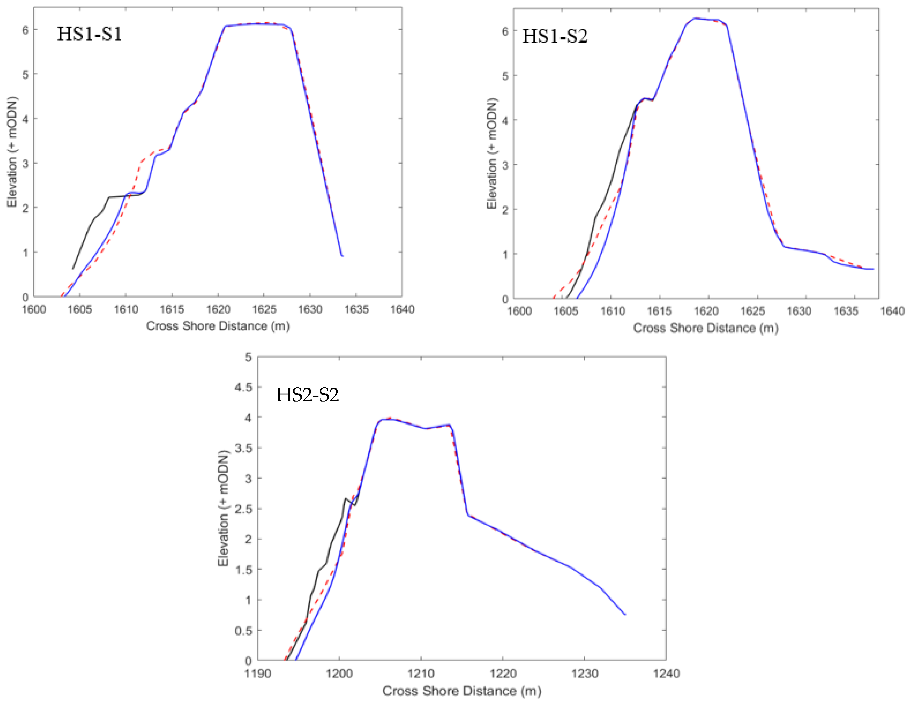
Figure 5 shows a comparison of measured and XBeach-simulated post-storm cross-shore profile response of the HCS for storm conditions given in Table 1, following model calibration. The majority of the profile change in those cases are seen in the middle and lower part of the profile while the upper beach remains unchanged. This may be due to wave run-up not reaching the upper beach. The model used gravel beach sediment transport formulation given in McCall et al. [20] and D50 of 15 mm and D90 of 45 mm [29]. To accurately quantify the comparisons, the Briers Skill Score (BSS) [40] and RMSE are utilised. The BSS categorises the model’s ability to correctly predict profile changes, where a score of 0–0.3 indicates ‘poor’ prediction, 0.3–0.6 indicates a ‘reasonable/fair’ model prediction, 0.6–0.8 indicates a ‘good’ score and lastly a score of 0.8–1.0 an excellent prediction. Both the skill score and RMSE were calculated using the profile change above 0 mODN due to the lack of accurate pre and post storm bathymetric measurements below 0 mODN available for storm calibration. Whilst morphological changes below the MSL dictate the evolution of the submerged beach step [15], the primary focus of this study was morphological change of the barrier crest above 0 mODN and therefore step dynamics are outside the scope of this study. The primary calibration parameters and the final selected values are given in Table 2. All selected parameter values were within the ranges recommended in the XBeach manual.
The calibration results reveal that the model is capable of satisfactorily capturing the morphodynamic response of the HCS gravel barrier to storms. Profile change at HS1-S1 case scored BSS of 0.62 and RMSE 0.24. HS1-S2 scored BSS of 0.6 and RMSE of 0.14 while HS2-S2 scored BSS of 0.78 and RMSE of 0.094, providing either ‘good’ or ‘excellent’ predictions. It should be noted that the model underpredicted the berm formation in HS1-S1 (Figure 5.) but the erosion of the lower beach is captured well. The model slightly overpredicted the erosion of the intertidal zone in HS1-S2 but upper beach, which is the most important areas in terms of barrier area change, is correctly modelled. In HS2-S2, the accretion of sediment on the upper beach area is captured very well although there was some overprediction of profile erosion in the lower beach area.
Direct validation of the HCS model against barrier overwash was not possible due to lack of overwash data. Therefore, the model was used to simulate if overwash occur at HS1 and HS2, during a series of storms given in Table 3 [6].
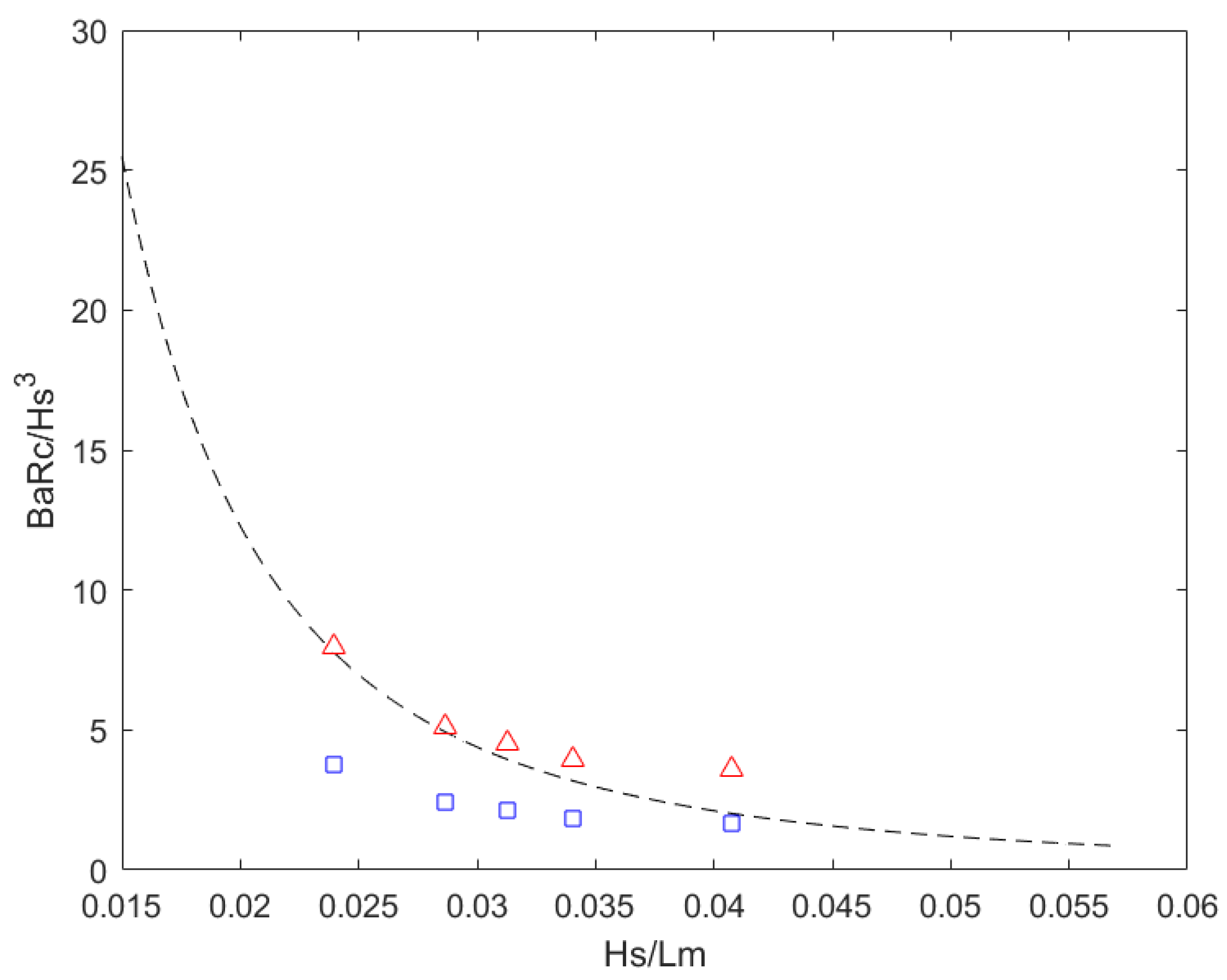
Using the Barrier Inertia Model (BIM) developed by Bradbury [9] and Bradbury et al. [6] given in Equation (7), which states that if the barrier inertia parameter is smaller than , overwashing will occur:
where Rc is barrier freeboard, Ba is barrier cross sectional area above MHWS + storm surge elevation (ESL), Hs is the significant storm wave height and Lm is deep water wavelength corresponding to mean wave period. Please refer to Figure 6 for definitions of variables. Using Equation (7), Bradbury et al. [6] estimated HS1 will not overwash during any of the storms given in Table 3 while HS2 will overwash during all storms except 1 in 1 year storm.
Figure 7 compares numerically simulated barrier inertia with Bradbury et al. [6] barrier inertia threshold at HS1 and HS2 from the 5 extreme storm conditions given in Table 3. At HS1, only the most severe storm event, 1:100, resulted in small amount of wave overtopping. In contrast, all storm events other than the 1:1 storm resulted in some overwashing or overtopping at HS2. Both results are in good agreement with the BIM, as shown in Figure 7, providing independent confirmation that the HCS model provides a reliable assessment of whether overwashing will occur during a storm.
3.3. Simulation of Gravel Beach Profile Change
In order to develop a simple parametric model to estimate gravel barrier profile change of a wide variety of gravel barrier beaches under storm conditions, the validated XBeach model was used to generate 880 barrier overwash and volume realisations. A range of barrier cross-sections and storm conditions were used. Synthetic storm conditions were developed following a statistical analysis of long-term wave measurements of the Milford wave buoy, described in Section 2. Fifteen statistically significant storm wave heights with varying return periods between 1:1 and 1:100 years, determined by Bradbury et al. [6], in which a Weibull distribution was fitted to 19 years of wave buoy data. JONSWAP unimodal spectrum was used to generate storm wave conditions. The duration of storms was kept constant at 20 h which is the mean storm duration calculated using storms derived from the wave data measured at Milford wave buoy. Storm threshold wave height of 2.74 m, defined by the CCO was used to isolate storms from the wave measurements [46].
Six extreme sea levels (ESL) levels with return periods 1:1, 1:10, 1:20, 1:50, 1:100 and 1:200 were derived from Coastal flood boundary conditions for UK mainland and islands (DEFRA 2018) [47]. Those were combined with tide data to determine total water levels. It was assumed that the storm peak and the peak storm surge occur at the highest tide. Five different barrier beach cross sections from HCS with varying shapes and crest elevations were selected. The storm conditions, water levels and profile shapes were then combined to generate 880 physically plausible realisations of input conditions (Table 4) to drive the XBeach model to simulate profile change and overwash. 36 realisations of bimodal storms with six different swell percentages were also generated using the data given in Table 4. Bimodal spectra to derive offshore storm boundary conditions to the XBeach model, were determined using the approach given by Polidoro and Dornbusch [48]. The significant wave height Hs for bimodal waves was determined using:
where is the significant wave height of the wind wave component and is the significant wave height of the swell wave component.
4. Results and Discussion
XBeach model simulations of gravel barrier overwashing and volume change were carried out for both unimodal and bimodal conditions explained in Section 3. Several modes of barrier response were observed (Figure 8), which have been categorised using the conceptual barrier response model of McCall et al. [20] (please note only the cross section change above + 0 mODN is shown):
- (1)
- Beach face erosion—For wave heights above the storm threshold height (2.74 m) combined with small peak wave periods (Tp < 11.5 s), where storm surge did not significantly reduce barrier freeboard (Rc), wave run up was confined to the swash zone. This resulted in sediment transported predominately offshore hence eroding the beach face (Figure 8A). Similar observations were found in Sallenger [49];
- (2)
- Crest accumulation—In cross sections with small freeboard and/or barrier area, crest build-up due to overtopping was observed under moderate storm conditions. A similar process was observed in profiles with larger freeboard under higher energy storm conditions. In both cases sediment was typically transported up the beach face due to an increased run-up and deposited on the barrier crest (Figure 8B). This process reduced the width of the barrier. Gravel sediment transport on beach face is well described by [15]. Bradbury and Powel [5] state that crest accumulation can occur when barrier is rolled over and, a new crest may form at a higher elevation and behind the original location of crest if there is sufficient sediment in the system. However, our results did not show evidence of this process;
- (3)
- Crest lowering—When energetic storm wave conditions (particularly with large wave periods) coincided with large surges, wave run-up exceeded the barrier freeboard and sediment was overwashed and deposited at the back of the barrier. As a result, the barrier crest was lowered and the width increased (Figure 8C). It was also observed that waves with low steepness increased overtopping. There were several cases where crest was lowered through avalanching of the barrier beach face;
- (4)
- Barrier Overwash—Once a barrier had started experiencing overwashing, the general trend was that an increase in surge, Hs and Tp resulted in more overwash, leading to more sediment being deposited further behind the barrier (Figure 8D). The larger values of Tp resulted in sediment deposited further away from the back of the barrier. If ESL is significantly large, overwashing occurred even during low wave energy conditions. When the most energetic storms combined with largest storm surges overwash sediment was deposited far behind the barrier thus losing sediment from the active barrier morphodynamic system. As a result, the barrier may be more vulnerable to future wave attack, with long term effect being landward translation of the barrier, unless coastal management interventions take place.
Other observations of barrier morphodynamic response were as follows: Barrier overtopping and/or overwashing was unlikely when both Ba and Rc are large; when Ba is large but Rc is small, the barrier was more prone to overwashing. Cases with a small Ba coupled with small Rc, experienced similar overwashing to that with large Ba and small Rc. This highlights the importance of Rc as an essential defence against extreme run-up that can occur during high surges. Ba appears to be of significance in controlling how soon the barrier becomes susceptible to overwashing events whereas smaller values of Ba can result in overwashing occurring earlier.
Bimodal impacts on HCS were found to be increase in barrier volume change and also, more importantly, altering the mode of barrier response. Where a barrier cross section was not previously susceptible to overwashing under unimodal conditions, bimodal conditions with high swell percentages with same energy were capable of producing severe overwashing events on the same barrier cross section.
To capture the change in barrier volume, an approach similar to Bradbury [9] was used by coupling key hydrodynamic and geometric variables. The extreme sea level, Hs and Tp were taken as the key hydrodynamic parameters while Ba, Rc and Zc (Figure 6) were taken as the key barrier geometric parameters. In order to better categorise the observed barrier responses using the controlling key parameters, a series of non-dimensional parameters were derived using parametric testing, which includes the Barrier inertia parameter of Bradbury [9] (hereafter known as Bi) given in Equation (9):
Bi has already been used to at numerous previous occasions to detect if barrier overwash is likely to occur on gravel beaches, as mentioned in Section 4. It includes the importance of surge level on barrier response, making it appropriate for use also in this study.
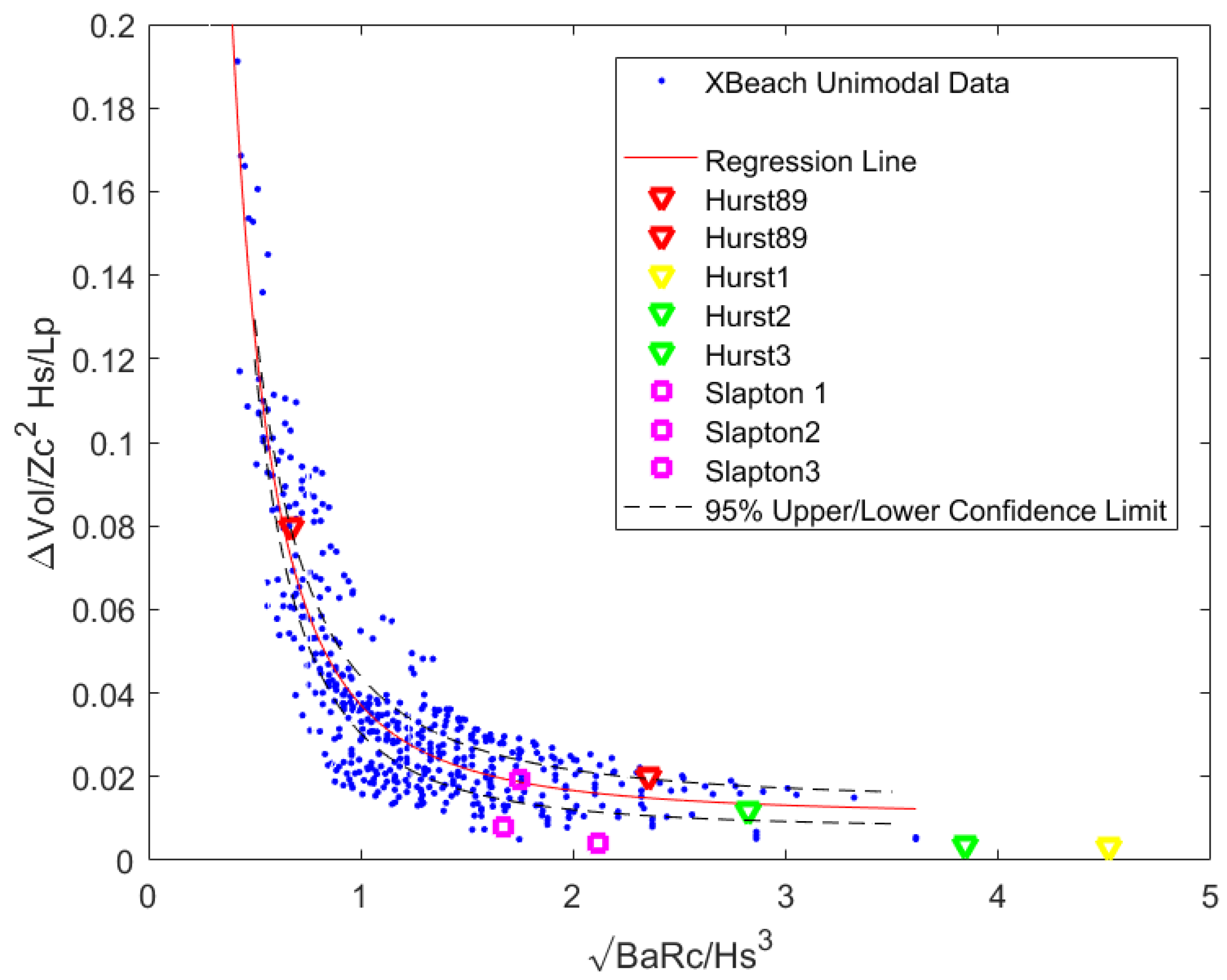
In Figure 9, the simulated non-dimensional barrier volume change above 0 m ODN per metre length of the barrier multiplied by wave steepness is shown against the square root of the barrier inertia parameter (Bi). The results show a clear trend where smaller Bi will give rise to larger barrier volume change as expected. The trendline derived using regression analysis and the 95% confidence intervals are also shown. The regression curve with r2 = 0.82 is given by the equation:
where ΔVol is volume change per metre width of the barrier and Lp is deep water wave length corresponding to peak wave period Tp.
The valid range of the regression equation should not exceed, which are the physical limits of conditions modelled in XBeachX:
and:
It may be useful if the regression curve given in Equation (10) can be used as a predictor to estimate change in barrier volume during storms, which can serve as a simple parametric model.
To check the validity of Equation (10) for conditions outside those used for numerical simulations, barrier volume change measured at several cross sections of HCS and the Slapton barrier beach located in the south-west of the UK during a range of storms were used (Table 5). The historic pre- and post-storm barrier cross sections and, storm wave and water level data are provided by the Channel Coastal Observatory of the UK, Bradbury [9], Bradbury et al. [6], McCall et al. [38] and Chadwick et al. [14].
The results reveal that two validation cases are outside the validity of Equation (10) . However, those cases resulted in very small barrier volume change and therefore, not significant. Four validation cases fell within the 95% confidence limits showing good degree of accuracy of the model while two cases were outside 95% confidence limit (Figure 9). Although further validation is necessary before the Equation (10) to be widely used as a parametric predictive model, these results give reasonable confidence to use it to estimate the changes in gravel barrier volume during storm events.
4.1. Simulated Bimodal Conditions Compared to Simulated Unimodal Conditions
Although the parametric model given in Equation (10) is derived based on numerically simulated barrier volume change during unimodal storm conditions, it is well known that the south-west of the UK is subjected to frequent storms with bimodal characteristics as a results of swell-dominated waves reaching from the Atlantic as mentioned in Section 2 [25,26,27]. To examine the impacts of bimodal storm conditions on gravel barriers, the model was used to simulate barrier volume change and overwash from bimodal storms explained in Section 3. In Figure 10 the non-dimensional barrier volume change from bimodal waves per metre length of the barrier are shown and compared with unimodal results. It can be seen that during bimodal storms with swell percentage greater than 40–50%, the non-dimensional barrier volume change for a given barrier inertia is larger than that from their unimodal counterparts, especially at low values of barrier inertia. There is a noticeable increase in barrier volume change from storms with 50% and 75% swell conditions. On the other hand, if the swell percentage is less than 30% non-dimensional barrier volume change is less than that from the unimodal cases for a given barrier inertia.
To examine the impact of wave bimodality on barrier response in more details, barrier volume change and overwash volume from storms under bimodal conditions at each individual cross section was investigated in isolation and compared with unimodal results. Figure 11 shows the results for cross section HS2, seen in Figure 4. Figure 11 clearly shows that the increasing swell wave component leads to greater barrier volume change and larger overwashing volumes and that when swell percentage is greater than 40% the barrier volume change and overwash volume is greater than that from the unimodal waves, for a given freeboard.
4.2. Simulation of Gravel Beach Sediment Overwash Volume
Gravel barrier beach overwashing is an important process which contributes to back barrier flooding as well as barrier response to storms. Therefore, the relationship between the overwashing volume and the barrier inertia parameter Bi was also investigated. Figure 12 gives the numerically simulated non-dimensional overwash volume from both unimodal and bimodal storm conditions. Although there is significant data scatter, an overall trend of overwash volume reduction with increase in barrier inertia can be seen. Also, similar to barrier volume change, overwash volumes from bimodal storms with higher swell percentages are significantly larger than that from unimodal storms for the same barrier inertia. During extreme cases where swell percentage is 75%, complete inundation of the barrier has taken place and a significant volume of sediment has been removed from the active barrier beach systems and transported further away from the back barrier. An event similar to this has been recorded at HCS where the barrier has breached following a storm in 2005 [25]. On the other hand, storms with less than 25% swell component gave rise to notably low overwash volumes.
A probable reason for ‘positive’ and ‘negative’ swell effects on the barrier volume change and overwashing may be explained by distinctly different behaviours of wind and swell waves. Short period wind waves dissipate further away from shore due to shoaling and steepening of the wave. This may limit the wave energy reaching the barrier beach face and wave run up. On the other hand, longer period swell waves, with their low wave steepness, can dominate the surf zone and propagate closer to the beach face without dissipation due to breaking [41,50]. If the swell percentage is small, wind waves dominate the surf, swash and runup while the contribution from swell waves may be small. For sea states with larger swell components, undissipated swell waves drive large runup and overtopping/overwashing. Polidoro et al. [13] observed that a swell percentage greater than 20% could have a larger impact on the elevation of the beach crest than the horizontal displacement of the beach, which agrees with our results.
5. Conclusions
The paper uses an extensive set of numerically simulated beach volume change and overwash data to developed a simple parametric model to estimate gravel barrier change under unimodal storm conditions and to investigate the response of gravel barriers to bimodal storm wave conditions. Following conclusions were drawn from the results:
- The XBeach non hydrostatic model is capable of simulating barrier volume change and overwash volume. The model was able to capture swash dynamics, sediment movement, barrier face erosion, crest build-up and back barrier sediment accumulation correctly, which was essential to the parametric model development in this study;
- The gravel barrier volume change during a collection of storms calculated using the parametric model were in good agreement with volume change measured in the field. This proves that the model will be a useful tool to estimate barrier volume change during storms, which can be taken as first estimates for coastal management purposes.
- Bimodal storm waves with large swell percentages (>50%) lead to greater barrier volume change and larger overwash volumes than their unimodal counterparts. This can be explained by the action of low steepness, high energy wave propagation on the slope of the barrier giving rise to higher runup and sediment movement on the face of the barrier.
- Following limitations of the approach are noted: Further validation of the parametric model is necessary to extend its application to a wide range of gravel barriers; the numerical simulations were carried out in 1D where the impacts of longshore transport were not taken into consideration; sea level change due to global warming is not considered in the simulations; and the parametric model may underestimate barrier volume change from bimodal storm conditions. Further studies will be carried out in the future to address those limitations.
Author Contributions
Conceptualization, H.K. and D.P.; Methodology, K.I., H.K. and D.P.; Validation K.I.; Formal Analysis, K.I. and H.K.; Investigation, K.I.; Resources, H.K., D.P.; Writing K.I. and H.K.; Writing—Review & Editing, H.K., D.E.R. and D.P.; Supervision, H.K. and D.P.; Project Administration, H.K.; Funding Acquisition, H.K. and D.P. All authors have read and agreed to the published version of the manuscript.
Funding
This research was funded by the Knowledge Economy Skills Scholarships (KESS II) which is a pan-Wales higher level skills initiative led by Bangor University on behalf of the Higher Education sector in Wales, UK and JBA Consulting.
Data Availability Statement
All results presented in this paper can be received upon request to the corresponding author. Data used can be accesses via UK Channel Coastal Observatory.
Acknowledgments
K.I. acknowledges the Knowledge Economy Skills Scholarships (KESS II) which is a pan-Wales higher level skills initiative led by Bangor University on behalf of the Higher Education sector in Wales, UK. The project was part funded by the Welsh Government’s European Social Fund (ESF) programme for East Wales and JBA Consulting enabling the pursuit of his MSc degree at Swansea University, UK. Channel Coastal Observatory is acknowledged for providing numerous data used in this study.
Conflicts of Interest
The authors declare no conflict of interest.
References
- Carter, R.W.G.; Orford, J.D.; Lauderdale, F.; Carter, R.W.G. The Morphodynamics of Coarse Clastic Beaches and Barriers: A Short- and Long-term Perspective. J. Coast. Res. 1993, 15, 158–179. [Google Scholar]
- Aminti, P.; Cipriani, L.E.; Pranzini, E. ‘Back to the Beach’: Converting Seawalls into Gravel Beaches. In Soft Shore Protection. Coastal Systems and Continental Margins; Goudas, C., Katsiaris, G., May, V., Karambas, T., Eds.; Springer: Dordrecht, The Netherlands, 2003; Volume 7. [Google Scholar] [CrossRef]
- Buscombe, D.; Masselinki, G. Concepts in gravel beach dynamics. Earth-Sci. Rev. 2006, 79, 33–52. [Google Scholar] [CrossRef]
- Almeida, L.P.; Masselink, G.; Russell, P.E.; Davidson, M.A. Observations of gravel beach dynamics during high energy wave conditions using a laser scanner. Geomorphology 2015, 228, 15–27. [Google Scholar] [CrossRef] [Green Version]
- Bradbury, A.P.; Powell, K.A. The Short Term Profile Response of Shingle Spits to Storm Wave Action. In Proceedings of the 23rd International Conference on Coastal Engineering, Venice, Italy, 4–9 October 1992; Volume 3, pp. 2694–2707. [Google Scholar]
- Bradbury, A.P.; Cope, S.N.; Prouty, D.B. Predicting the response of shingle barrier beaches under extreme wave and water level conditions in southern England. In Coastal Dynamics 2005; American Society of Civil Engineers: Reston, VA, USA, 2005. [Google Scholar]
- Powell, K.A. The dynamic response of shingle beaches to random waves. In Proceedings of the 21st International Conference on Coastal Engineering, Malaga, Spain, 20–25 June 1988; pp. 1763–1773. [Google Scholar]
- Powell, K.A. Predicting Short-Term Profile Response for Shingle Beaches; Hydraulics Research Report SR219; HR Wallingford: Wallingford, UK, 1990. [Google Scholar]
- Bradbury, A.P. Predicting breaching of shingle barrier beaches-recent advances to aid beach management. In Proceedings of the 35th Annual MAFF Conference of River and Coastal Engineers, London, UK, July 2000; Available online: https://www.semanticscholar.org/paper/PREDICTING-BREACHING-OF-SHINGLE-BARRIER-ADVANCES-TO-Bradbury/ee91f390d2c45f6a0f99b31e5fb1e858213b87f3 (accessed on 17 December 2019).
- de San Román-Blanco, B.L.; Coates, T.T.; Holmes, P.; Chadwick, A.J.; Bradbury, A.; Baldock, T.E.; Pedrozo-Acuña, A.; Lawrence, J.; Grüne, J. Large scale experiments on gravel and mixed beaches: Experimental procedure, data documentation and initial results. Coast. Eng. 2006, 53, 349–362. [Google Scholar] [CrossRef]
- Van Rijn, L.C.; Sutherland, J.; Rosati, J.D.; Wang, P.; Roberts, T.M. Erosion of gravel barriers and beaches. In Proceedings of the Coastal Sediments 2011, Miami, FL, USA, 2–6 May 2011. [Google Scholar]
- Matias, A.; Blenkinsopp, C.E.; Masselink, G. Detailed investigation of overwash on a gravel barrier. Mar. Geol. 2014, 350, 27–38. [Google Scholar] [CrossRef] [Green Version]
- Polidoro, A.; Pullen, T.; Eade, J.; Mason, T.; Blanco, B.; Wyncoll, D. Gravel beach profile response allowing for bimodal sea states. Proc. Inst. Civ. Eng. Marit. Eng. 2018, 171, 145–166. [Google Scholar] [CrossRef]
- Chadwick, A.J.; Karunarathna, H.; Gehrels, W.R.; Massey, A.C.; O’Brien, D.; Dales, D. A new analysis of the Slapton barrier beach system, UK. Proc. Inst. Civ. Eng. Marit. Eng. 2005, 158, 147–161. [Google Scholar] [CrossRef]
- Austin, M.J.; Buscombe, D. Morphological change and sediment dynamics of the beach step on a macrotidal gravel beach. Mar. Geol. 2008, 249, 167–183. [Google Scholar] [CrossRef]
- de Alegria-Arzaburu, A.R.; Masselink, G. Storm response and beach rotation on a gravel beach, Slapton Sands, UK. Mar. Geol. 2010, 278, 77–99. [Google Scholar] [CrossRef]
- Williams, J.J.; De Alegria-Arzaburu, A.R.; McCall, R.T.; Van Dongeren, A.; Van Dongeren, A. Modelling gravel barrier profile response to combined waves and tides using XBeach: Laboratory and field results. Coast. Eng. 2012, 63, 62–80. [Google Scholar] [CrossRef]
- Roelvink, D.; Reniers, A.; Van Dongeren, A.; van Thiel de Vries, J.; McCall, R.; Lescinski, J. Modelling storm impacts on beaches, dunes and barrier islands. Coast. Eng. 2009, 56, 1133–1152. [Google Scholar] [CrossRef]
- Jamal, M.H.; Simmonds, D.J.; Magar, V. Modelling gravel beach dynamics with XBeach. Coast. Eng. 2014, 89, 20–29. [Google Scholar] [CrossRef]
- McCall, R.T.; Masselink, G.; Poate, T.G.; Roelvink, D.; Almeida, L.P. Modelling the morphodynamics of gravel beaches during storms with XBeach-G. Coast. Eng. 2015, 103, 52–66. [Google Scholar] [CrossRef]
- Gharagozlou, A.; Dietrich, J.C.; Karanci, A.; Luettich, R.A.; Overton, M.F. Storm-driven erosion and inundation of barrier islands from dune-to region-scales. Coast. Eng. 2020, 158, 103674. [Google Scholar] [CrossRef]
- Phillips, B.T.; Brown, J.M.; Plater, A.J. Modeling Impact of Intertidal Foreshore Evolution on Gravel Barrier Erosion and Wave Runup with Xbeach-X. J. Mar. Sci. Eng. 2020, 8, 914. [Google Scholar] [CrossRef]
- Roelvink, D.; McCall, R.; Mehvar, S.; Nederhoff, K.; Dastgheib, A. Improving predictions of swash dynamics in XBeach: The role of groupiness and incident-band runup. Coast. Eng. 2018, 134, 103–123. [Google Scholar] [CrossRef]
- Poate, T.G.; McCall, R.T.; Masselink, G. A new parameterisation for runup on gravel beaches. Coast. Eng. 2016, 117, 176–190. [Google Scholar] [CrossRef] [Green Version]
- Bradbury, A.P.; Mason, T.E.; Poate, T. Implications of the spectral shape of wave conditions for engineering design and coastal hazard assessment—Evidence from the English Channel. In Proceedings of the 10th International Workshop on Wave Hindcasting and Forecasting and Coastal Hazard Symposium, North Shore, Oahu, HI, USA, 11–16 November 2007; pp. 1–17. [Google Scholar]
- Thompson, D.A.; Karunarathna, H.; Reeve, D.E. An Analysis of Swell and Bimodality around the South and South-west coastline of England. Nat. Hazards Earth Syst. Sci. Discuss. 2018. Available online: https://nhess.copernicus.org/preprints/nhess-2018-117/ (accessed on 17 December 2019). [CrossRef]
- Nicholls, R.; Webber, N. Characteristics of Shingle Beaches with Reference to Christchurch Bay, S. England. In Proceedings of the 21st International Conference on Coastal Engineering, Malaga, Spain, 20–25 June 1988; pp. 1922–1936. [Google Scholar] [CrossRef]
- British Oceanography Data Centre BODC. Available online: https://www.bodc.ac.uk/data/hosted_data_sys-tems/sea_level/uk_tide_gauge_network/ (accessed on 18 January 2020).
- Bradbury, A.P.; Kidd, R. Hurst spit stabilisation scheme. Design and construction of beach recharge. In Proceedings of the 33rd MAFF Conference of River and Coastal Engineers, Keele, UK, 1–3 July 1998; Volume 1. No. 1. [Google Scholar]
- Nicholls, R. The Stability of Shingle Beaches in the Eastern Half of Christchurch Bay. Unpublished Ph.D. Thesis, Department of Civil Engineering, University of Southampton, Southampton, UK, 1985; 468p. [Google Scholar]
- Bradbury, A.P. Evaluation of coastal process impacts arising from nearshore aggregate dredging for beach re-charge—Shingles Banks, Christchurch Bay. In Proceedings of the International Conference on Coastal Manage-ment 2003, Brighton, UK, 15–17 October 2003; pp. 1–15. [Google Scholar]
- Channel Coastal Observatory (CCO). Available online: https://www.channelcoast.org/ (accessed on 18 January 2020).
- Williams, J.J.; Esteves, L.S.; Rochford, L.A. Modelling storm responses on a high-energy coastline with XBeach. Model. Earth Syst. Environ. 2015, 1, 1–14. [Google Scholar] [CrossRef] [Green Version]
- Holthuijsen, L.H.; Booij, N.; Herbers, T.H.C. A prediction model for stationary, short-crested waves in shallow water with ambient currents. Coast. Eng. 1989, 13, 23–54. [Google Scholar] [CrossRef]
- Smit, P.B.; Roelvink, J.A.; van Thiel de Vries, J.S.M.; McCall, R.T.; van Dongeren, A.R.; Zwinkels, J.R. XBeach Manual: Non-Hydrostatic Model. Validation, Verification and Model Description; Delft University of Technology: Delft, The Netherlands, 2010. [Google Scholar]
- Smit, P.; Zijlema, M.; Stelling, G. Depth-induced wave breaking in a non-hydrostatic, near-shore wave model. Coast. Eng. 2013, 76, 1–16. [Google Scholar] [CrossRef]
- Zijlema, M.; Stelling, G.; Smit, P. SWASH: An operational public domain code for simulating wave fields and rapidly varied flows in coastal waters. Coast. Eng. 2011, 58, 992–1012. [Google Scholar] [CrossRef]
- McCall, R.; Masselink, G.; Poate, T.; Bradbury, A.; Russell, P.; Davidson, M. Predicting overwash on gravel barri-ers. J. Coast. Res. 2013, 1473–1478. [Google Scholar] [CrossRef]
- McCall, R.T.; Masselink, G.; Poate, T.G.; Roelvink, J.A.; Almeida, L.P.; Davidson, M.; Russell, P.E. Modelling storm hydrodynamics on gravel beaches with XBeach-G. Coast. Eng. 2014, 91, 231–250. [Google Scholar] [CrossRef] [Green Version]
- Van Rijn, L.C.; Walstra, D.J.R.; Grasmeijer, B.; Sutherland, J.; Pan, S.; Sierra, J.P. The predictability of cross-shore bed evolution of sandy beaches at the time scale of storms and seasons using process-based Profile models. Coast. Eng. 2003, 47, 295–327. [Google Scholar] [CrossRef]
- Masselink, G.; McCall, R.; Poate, T.; Van Geer, P. Modelling storm response on gravel beaches using XBeach-G. Proc. Inst. Civ. Eng. Marit. Eng. 2014, 167, 173–191. [Google Scholar] [CrossRef] [Green Version]
- Orimoloye, S.; Karunarathna, H.; Reeve, D.E. Effects of swell on wave height distribution of energy-conserved bimodal seas. J. Mar. Sci. Eng. 2019, 7, 79. [Google Scholar] [CrossRef] [Green Version]
- Soulsby, R.L.; Whitehouse, R.J.S. Threshold of sediment motion in coastal environments. In Pacific Coasts and Ports’ 97: Proceedings of the 13th Australasian Coastal and Ocean Engineering Conference and the 6th Australasian Port and Harbour Conference; Centre for Advanced Engineering, University of Canterbury: Christchurch, New Zealand, 1997; Volume 1. [Google Scholar]
- Van Rijn, L.C. Unified View of Sediment Transport by Currents and Waves. III: Graded Beds. J. Hydraul. Eng. 2007, 133, 761–775. [Google Scholar] [CrossRef] [Green Version]
- Van Rijn, L.C. Principles of Sediment Transport in Rivers, Estuaries and Coastal Seas; Aqua Publications: Amsterdam, The Netherlands, 1993; Volume 1006. [Google Scholar]
- XBeach Manual, Model Description and Reference Guide to Functionalities, Deltares. 2015. Available online: https://xbeach.readthedocs.io/en/latest/xbeach_manual (accessed on 17 December 2019).
- Department for Environment, Food and Rural Affairs (DEFRA) DE-FRA. Available online: https://www.gov.uk/government/organisations/department-for-environment-food-rural-affairs (accessed on 17 December 2019).
- Polidoro, A.; Dornbusch, U. Wave Run-Up on Shingle Beaches—A New Method; HR Wallingford Technical Report CAS0942-RT001-R05-00; HR Wallingford: Wallingford, UK, 2014. [Google Scholar]
- Sallenger, A.H., Jr. Storm impact scale for barrier islands. J. Coast. Res. 2000, 16, 890–895. [Google Scholar]
- Almeida, L.P.; Masselink, G.; McCall, R.; Russell, P. Storm overwash of a gravel barrier: Field measurements and XBeach-G modelling. Coast. Eng. 2017, 120, 22–35. [Google Scholar] [CrossRef] [Green Version]
Figure 1.
Location of Study, Hurst Spit Beach SW England located in the English Channel, UK (Google Earth).
Figure 1.
Location of Study, Hurst Spit Beach SW England located in the English Channel, UK (Google Earth).

Figure 2.
(Top image)—Hurst Spit aerial photograph, showing salt marshes and Hurst Castle located at the end of the spit (Channel Coastal Observatory). (Bottom image)—Hurst Spit Beach, showing gravel composition of the beach.
Figure 2.
(Top image)—Hurst Spit aerial photograph, showing salt marshes and Hurst Castle located at the end of the spit (Channel Coastal Observatory). (Bottom image)—Hurst Spit Beach, showing gravel composition of the beach.

Figure 3.
Nearshore bathymetry of Hurst Castle Spit gravel barrier beach and the surroundings. Bathymetry data are from Channel Coastal Observatory.
Figure 3.
Nearshore bathymetry of Hurst Castle Spit gravel barrier beach and the surroundings. Bathymetry data are from Channel Coastal Observatory.

Figure 4.
Cross sections of the Hurst Castle Spit gravel barrier beach used for model calibration and their locations. Locations (left) and cross section profiles (right), where left side of the figures are seaward and the right side of the figure is landward.
Figure 4.
Cross sections of the Hurst Castle Spit gravel barrier beach used for model calibration and their locations. Locations (left) and cross section profiles (right), where left side of the figures are seaward and the right side of the figure is landward.

Figure 5.
A comparison of measured and simulated post-storm profiles (HS1-top and HS2-bottom) at HCS following XBeachX model calibration against storms S1 and S2. Measured pre-storm profile (—black line), measured post-storm profile (—red dotted line) and simulated post-storm profile (—blue line).
Figure 5.
A comparison of measured and simulated post-storm profiles (HS1-top and HS2-bottom) at HCS following XBeachX model calibration against storms S1 and S2. Measured pre-storm profile (—black line), measured post-storm profile (—red dotted line) and simulated post-storm profile (—blue line).

Figure 6.
Schematisation of barrier geometry. Ba = pre-storm barrier cross sectional area above Surge level mODN + MHWS, Rc = initial barrier freeboard and Zc = initial barrier crest height.
Figure 6.
Schematisation of barrier geometry. Ba = pre-storm barrier cross sectional area above Surge level mODN + MHWS, Rc = initial barrier freeboard and Zc = initial barrier crest height.

Figure 7.
Comparison of Bradbury [9] and Bradbury et al. [6] Barrier Inertia Model and XBeach simulations. Black broken line-overwash threshold given by barrier inertia threshold of Bradbury [9]. Red triangles and blue squares are XBeach simulations at HS1 to HS2, respectively.

Figure 8.
Observed morphodynamic responses of the barrier beach to storm events, from the simulated results. Black line-Pre-storm, Blue line-Post-storm. (A) Beach face erosion; (B) Crest accumulation; (C) Crest lowering; and (D) Barrier overwash.
Figure 8.
Observed morphodynamic responses of the barrier beach to storm events, from the simulated results. Black line-Pre-storm, Blue line-Post-storm. (A) Beach face erosion; (B) Crest accumulation; (C) Crest lowering; and (D) Barrier overwash.

Figure 9.
Non-dimensional barrier volume change above 0 m ODN per metre length of the barrier a during storm against the square root of the barrier inertia parameter (Bi). The exponential regression trendline is given by the red curve. 95% confidence limits are shown by the broken black curve. The regression curve validation data at HCS and Slapton Barrier beach are shown in green, yellow and red triangles and purple squares.

Figure 10.
Comparison of unimodal and bimodal non-dimensional barrier volume change under different swell percentages. The red curve is the parametric model given by Equation (10).
Figure 10.
Comparison of unimodal and bimodal non-dimensional barrier volume change under different swell percentages. The red curve is the parametric model given by Equation (10).

Figure 11.
The effect of swell percentage of bimodal storm waves on barrier volume change (left) and overwash volume (right) for a single cross section, HS2. Δvol = barrier volume change per metre length and Vol = pre-storm barrier volume/metre length; OV = overwash volume.
Figure 11.
The effect of swell percentage of bimodal storm waves on barrier volume change (left) and overwash volume (right) for a single cross section, HS2. Δvol = barrier volume change per metre length and Vol = pre-storm barrier volume/metre length; OV = overwash volume.

Figure 12.
A comparison of simulated barrier overwash volumes from unimodal storms and bimodal storms with varying swell percentages.
Figure 12.
A comparison of simulated barrier overwash volumes from unimodal storms and bimodal storms with varying swell percentages.


Table 1.
HCS gravel barrier cross-sections and storm conditions extracted from the Milford wave buoy for model calibration, used for XBeach model validation. (Hs)max = maximum significant wave height; Tp = peak wave period from the JONSWAP spectrum; θ = wave approach direction from the north; MHWS = mean high water spring during the storm. S1—storm 1, S2—storm 2.
| Cross Section | Crest Height m ODN | Pre-Storm Profile Date | Post-Storm Profile Date | Storm Duration (h) | (Hs)max (m) | Tp (s) | θ | MHWS above ODN (m) |
|---|---|---|---|---|---|---|---|---|
| HS1-S1 | 6.27 | 28/10/2011 | 31/10/2011 | 10 (S1) | 2.75 | 18 | 220 | 1.1 |
| HS1-S2 | 6.27 | 09/11/2011 | 13/11/2011 | 24 (S2) | 3.85 | 8.3 | 216 | 0.928 |
| HS2-S2 | 3.96 | 09/11/2011 | 13/11/2011 | 24 (S2) | 3.85 | 8.3 | 216 | 0.928 |
Table 2.
Calibration parameters of the XBeach non-hydrostatic model of the Hurst Castle Spit gavel barrier beach and the final selected values which gave the best fit profile with measured profile. dryslp is critical avalanching slope above water level, wetslp is critical avalanching slope below water level, CFL is maximum courant Friedrichs-Lewy number, repose angle is the angle of internal friction of sediment, kx is hydraulic gradient, ci is mass coefficient in shields inertia term, morfac is the morphological acceleration factor and cf is the bed friction factor.
| Model Parameter | Recommended Range | Default Value | Selected Value |
|---|---|---|---|
| dryslp | 0.1–2.0 | 1.0 | 1.0 |
| wetslp | 0.1–1.0 | 0.3 | 0.3 |
| CFL | 0.7–0.9 | 0.7 | 0.9 |
| reposeangle | 0–45 | 30 | 45 |
| kx | 0.01–0.3 | 0.01 | 0.15 |
| ci | 0.5–1.5 | 1.0 | 1.0 |
| morfac | 1–1000 | 1 | 1 |
| Cf | 3D90 | 3D90 | 3D90 |
Table 3.
Storm conditions used to model barrier overwash for comparison with Bradbury et al. [6] results.
Table 3.
Storm conditions used to model barrier overwash for comparison with Bradbury et al. [6] results.
| Storm Return Period | Hs (m) | Tm (s) | Storm Surge Imposed on MHWS (m) |
|---|---|---|---|
| 1:1 | 3.69 | 8.64 | 1.0 |
| 1:10 | 4.22 | 9.30 | 1.0 |
| 1:20 | 4.39 | 9.48 | 1.0 |
| 1:50 | 4.6 | 9.71 | 1.0 |
| 1:100 | 4.75 | 9.87 | 1.0 |
Table 4.
Significant wave heights, peak periods and storm surges with a range of return periods used to generate synthetic unimodal and bimodal storm events.
Table 4.
Significant wave heights, peak periods and storm surges with a range of return periods used to generate synthetic unimodal and bimodal storm events.
| Unimodal Cases | Bimodal Cases | ||||
|---|---|---|---|---|---|
| Hs (m) | Tp (s) | MHWS + Surge above ODN (ESL) (m) | Hs (Bimodal) (m) | MHWS + Surge above ODN (ESL) (m) | Swell Percentage |
| 2.75, 2.94, 3.13, 3.31, 3.50, 3.64, 3.76, 3.87, 3.99, 4.11, 4.22, 4.34, 4.46, 4.57, 4.69, 4.75 | 8.0, 9.0, 10.0, 11.5 | 1.52, 1.80, 1.96, 2.07, 2.20, 2.40 | 2.75, 3.64, 4.10, 4.75 | 1.52, 1.80, 1.96, 2.07, 2.20, 2.40 | 10, 25, 35, 40, 50, 75 |
Table 5.
Volume change measured at cross sections along HCS and Slapton beach during storm events, used to validate Equation (10).
Table 5.
Volume change measured at cross sections along HCS and Slapton beach during storm events, used to validate Equation (10).
| Validation Case | Hs (m) | Tp (s) | Water Level above ODN (m) (ESL) |
|---|---|---|---|
| Hurst 89 | 2.9 | 10.96 | 0.87 |
| Hurst 89 | 2.9 | 10.96 | 0.87 |
| Hurst 1 | 3 | 12.6 | 1 |
| Hurst 2 | 3.95 | 12.3 | 1.27 |
| Hurst3 | 3.95 | 12.3 | 1.27 |
| Slapton 1 | 4.87 | 8.3 | 1.905 |
| Slapton 2 | 4.87 | 8.3 | 1.905 |
| Slapton 3 | 4.87 | 8.3 | 1.905 |
Publisher’s Note: MDPI stays neutral with regard to jurisdictional claims in published maps and institutional affiliations. |
© 2021 by the authors. Licensee MDPI, Basel, Switzerland. This article is an open access article distributed under the terms and conditions of the Creative Commons Attribution (CC BY) license (http://creativecommons.org/licenses/by/4.0/).
Share and Cite
MDPI and ACS Style
Ions, K.; Karunarathna, H.; Reeve, D.E.; Pender, D. Gravel Barrier Beach Morphodynamic Response to Extreme Conditions. J. Mar. Sci. Eng. 2021, 9, 135. https://doi.org/10.3390/jmse9020135
AMA Style
Ions K, Karunarathna H, Reeve DE, Pender D. Gravel Barrier Beach Morphodynamic Response to Extreme Conditions. Journal of Marine Science and Engineering. 2021; 9(2):135. https://doi.org/10.3390/jmse9020135
Chicago/Turabian StyleIons, Kristian, Harshinie Karunarathna, Dominic E. Reeve, and Douglas Pender. 2021. "Gravel Barrier Beach Morphodynamic Response to Extreme Conditions" Journal of Marine Science and Engineering 9, no. 2: 135. https://doi.org/10.3390/jmse9020135
Note that from the first issue of 2016, this journal uses article numbers instead of page numbers. See further details here.