Article

A Novel Zeroing Neural Network for Solving Time-Varying Quadratic Matrix Equations against Linear Noises

1
College of Computer Science and Engineering, Jishou University, Jishou 416000, China
2
Department of Computer Science, Swansea University, Swansea SA1 8EN, UK
3
Department of Mechanical Engineering, Swansea University, Swansea SA1 8EN, UK
4
College of Mathematics and Statistics, Jishou University, Jishou 416000, China
*
Author to whom correspondence should be addressed.
Mathematics 2023, 11(2), 475; https://doi.org/10.3390/math11020475
Submission received: 13 December 2022 / Revised: 7 January 2023 / Accepted: 13 January 2023 / Published: 16 January 2023

Abstract

:
The solving of quadratic matrix equations is a fundamental issue which essentially exists in the optimal control domain. However, noises exerted on the coefficients of quadratic matrix equations may affect the accuracy of the solutions. In order to solve the time-varying quadratic matrix equation problem under linear noise, a new error-processing design formula is proposed, and a resultant novel zeroing neural network model is developed. The new design formula incorporates a second-order error-processing manner, and the double-integration-enhanced zeroing neural network (DIEZNN) model is further proposed for solving time-varying quadratic matrix equations subject to linear noises. Compared with the original zeroing neural network (OZNN) model, finite-time zeroing neural network (FTZNN) model and integration-enhanced zeroing neural network (IEZNN) model, the DIEZNN model shows the superiority of its solution under linear noise; that is, when solving the problem of a time-varying quadratic matrix equation in the environment of linear noise, the residual error of the existing model will maintain a large level due to the influence of linear noise, which will eventually lead to the solution’s failure. The newly proposed DIEZNN model can guarantee a normal solution to the time-varying quadratic matrix equation task no matter how much linear noise there is. In addition, the theoretical analysis proves that the neural state of the DIEZNN model can converge to the theoretical solution even under linear noise. The computer simulation results further substantiate the superiority of the DIEZNN model in solving time-varying quadratic matrix equations under linear noise.

1. Introduction

The quadratic matrix equation (QME), as a fundamental nonlinear paradigm, arises frequently in a variety of applications. The application of the QME extensively appears in optimal control [1,2,3], the analysis of structural systems and vibration problems [4,5,6,7,8,9], block tridiagonal transition probability matrices which are used in two-dimensional Markov chains with quasi-birth-death processes [10,11], damped mass-spring systems [11], telecommunication stochastic models [12], computer performance and inventory control [13]. To solve the QME, many techniques have been proposed and investigated [11,14,15,16,17,18,19,20]. For instance, Davis [14,15] used Newton’s method to solve the QME, with theoretical analysis and implementation details provided. Benner and Byers [16] studied the use of exact line searching in Newton’s methods for solving algebraic Riccati equations, which are a special type of QME. Higham et al. [11] solved the QME with the Bernoulli iterative method and a convergence time less than that in Newton’s methods.
The aforementioned approaches were instinctively designed to solve static QMEs in a serial processing manner. In recent years, dynamic solvers with a parallel processing ability have been developed and attracted attention from research communities [21,22,23]. The neural dynamic method can be a strong alternative for matrix computation problems due to its parallelism and ease of hardware implementation. For example, the GNNs [24,25,26] that evolve along the negative gradient descent direction of the scalar-valued energy function cause the residual errors to gradually approach zero over time. However, even after an infinite amount of time, the GNN model cannot converge to the exact solution under time-varying situations; it can only arrive at an approximation of the theoretical solution of the time-varying matrix. This is because the GNNs do not use the time derivative information of the coefficient matrix or there is a lack of velocity compensation for the time-varying coefficient. As a special kind of recurrent neural network solver, zeroing neural networks (ZNNs) have recently been developed and applied in various time-varying matrix problems in an online manner [27,28,29,30,31]. Compared with the GNNs, a ZNN makes full use of the time derivative of the time-varying term for superior convergence performance. Furthermore, the ZNN model can be effectively applied to different types of redundant robot manipulators. For example, the Li function-activated zeroing neural network (LFAZNN) has been applied to the four-link planar manipulator and PA10 manipulator [32], and the integration-enhanced zeroing neural network (IEZNN) has been applied to the two-link planar robot manipulator [33].
Various internal and external noises are not considered primitively in the design and implementation of dynamic recurrent neural networks, such as the OZNN model for the solution of a time-varying matrix square root [34,35] or the FTZNN model for the solution of a time-varying matrix square root [36]. These models can be solved effectively in a noiseless environment, and the network state solution of the neural network model can converge to the theoretical solution of the square root of the time-varying matrix. However, the neural network models could be contaminated by implementation errors when they are applied to computational issues. Eventually, accurate solutions may not be found under such unexpected exerted noises. As noises may always appear and exist in the coefficients of the neural network models after the solution process, involving the denoising loop and pretreating noises prior to the solution process can be time-consuming and unnecessary. Therefore, it is crucial to diminish the negative effects of noise during the solution. The IEZNN model shows excellent convergence performance when solving the time-varying matrix inverse with constant noise interference, but when there is linear noise interference, the IEZNN model cannot completely suppress linear noise, and the residual error of the IEZNN model cannot converge to zero [33].
In this paper, in order to solve the time-varying QME under simultaneous linear noise, a novel ZNN model with a double-integrated enhanced error-processing loop is proposed and studied. Such a model, termed as the DIEZNN, is able to make its neural state converge to the theoretical solution globally even under linear noise. The proposed DIEZNN model can be substantiated to possess improved convergence performance compared with other state-of-the-art models; that is, unbounded linear noise will greatly affect the solving ability of existing models, and the DIEZNN model proposed can suppress this unbounded linear noise well. In other words, when solving the time-varying QME under linear noise, the neural state solution of the DIEZNN model can converge to the theoretical solution of the time-varying QME, and the residual error of the DIEZNN model can be kept very small. The efficiency of the model is further verified by example computational results.
The rest of this paper is organized into the following sections. The problem formulation is presented in Section 2. The dynamic recurrent neural network method is presented in Section 3. In Section 4, the theoretical analysis and results are addressed to investigate the convergence properties of the DIEZNN model for the solution of the time-varying QME without and with linear noise. Section 5 provides three experimental examples to verify the superiority of the DIEZNN model compared with other existing models. The conclusion is given in Section 6. The main contributions of this paper are listed below:
  • In order to suppress linear noise perturbation for the solution of the time-varying QME, a DIEZNN model is first proposed with a new error-processing method.
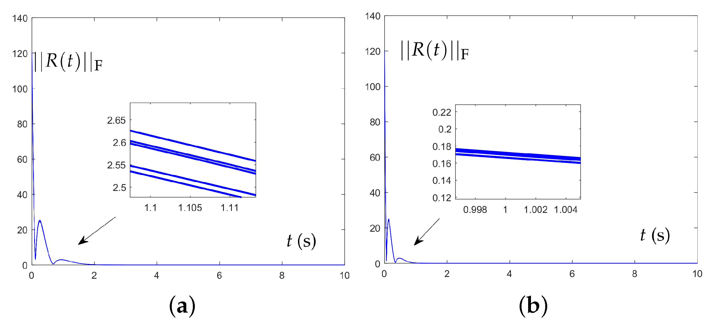
  • Theoretical analysis demonstrates that the proposed DIEZNN model converges to the theoretical solution of the QME globally. More importantly, the DIEZNN model is proved to also be able to converge to the theoretical solution of the QME in the case of linear noise interference.
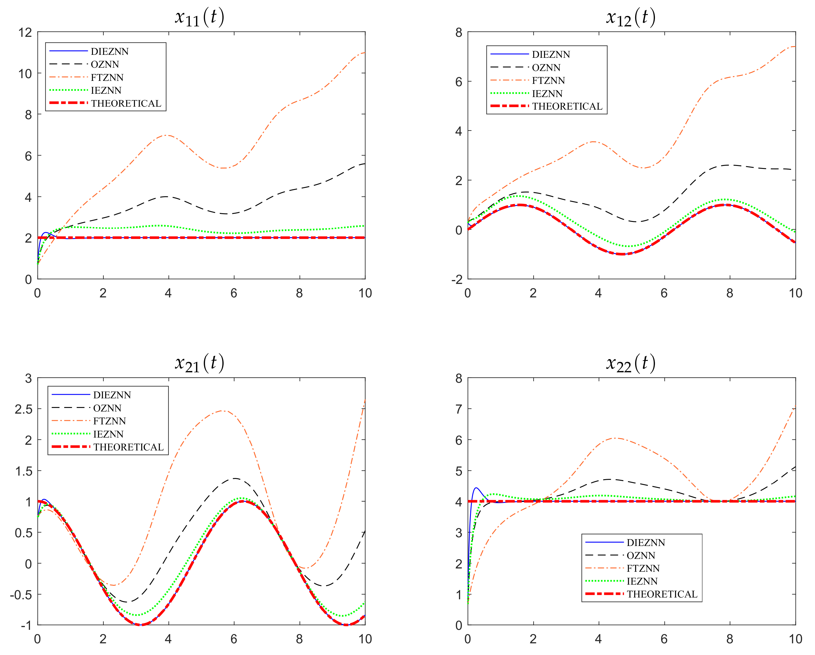
  • The superiority of the DIEZNN model to solve the time-varying QME under linear noise, compared with other methods such as the OZNN, FTZNN and IEZNN, is further verified by three simulation examples.

2. Problem Formulation

In this section, the problem formulation of time-varying QME subject to noise is presented first. Afterward, the proposed novel DIEZNN model with other comparative models is addressed. In this work, let us consider the following time-varying QME:
A ( t ) X 2 ( t ) + B ( t ) X ( t ) + C ( t ) = 0 .
where X ( t ) R n × n denotes an unknown time-varying matrix to be obtained, A ( t ) R n × n , B ( t ) R n × n and C ( t ) R n × n are known time-varying matrices and X * ( t ) denotes the theoretical solution to Equation (1). We assume that A ( t ) , B ( t ) and C ( t ) are non-singular at any time ( t 0 , ) and the A ( t ) , B ( t ) and C ( t ) time derivatives are uniformly bounded.
When the noises come into the time-varying QME (Equation (1)), it further becomes
( A ( t ) + Δ A ( t ) ) X 2 ( t ) + ( B ( t ) + Δ B ( t ) ) X ( t ) + C ( t ) + Δ C ( t ) = 0 ,
where Δ A ( t ) , Δ B ( t ) and Δ C ( t ) are noise disturbances to the time-varying coefficients. The accurate solution of the time-varying QME (Equation (1)) will be perturbed by the degraded model with coefficient noise. In this work, we propose to solve such a time-varying QME under linear noise with our newly developed DIEZNN models.

3. Dynamic Recurrent Neural Network Method

3.1. OZNN Model

When the GNN model is used to solve the time-varying problem, only the approximate solution of the time-varying problem can be obtained, and it cannot converge to the exact solution of the time-varying matrix problem while the residual error cannot converge to zero [24]. Moreover, the residual error of the GNN model is larger when it is used to solve time-varying problems under linear noise conditions [33].
For comparative purposes, other models are presented to show the differences with the proposed DIEZNN model. In order to solve the time-varying QME with linear noise, instead of using a GNN model, the original zeroing neural network (OZNN) model needs to process the error as follows:
R ( t ) = ( A ( t ) + Δ A ( t ) ) X 2 ( t ) + ( B ( t ) + Δ B ( t ) ) X ( t ) + C ( t ) + Δ C ( t ) .
In order to make R ( t ) approach zero as time evolves, the following error processing formula is adopted [24]:
R ˙ ( t ) = γ R ( t )
By expanding the design formula, the OZNN model for solving the time-varying QME under linear noise is derived as follows:
( A ( t ) + Δ A ( t ) ) X ˙ ( t ) X ( t ) + ( ( A ( t ) + Δ A ( t ) ) X ( t ) + B ( t ) + Δ B ( t ) ) X ˙ ( t ) = ( ( A ˙ ( t ) + Δ A ˙ ( t ) ) X ( t ) + B ˙ ( t ) + Δ B ˙ ( t ) ) X ( t ) C ˙ ( t ) Δ C ˙ ( t ) γ ( ( ( A ( t ) + Δ A ( t ) ) X ( t ) + B ( t ) + Δ B ( t ) ) X ( t ) + C ( t ) + Δ C ( t ) ) .
where γ denotes the design parameters to control the convergence rate.

3.2. FTZNN Model

To solve for the time-varying matrix QME with linear noise, the following error function is applied to the finite-time zeroing neural network (FTZNN) model:
R ( t ) = ( A ( t ) + Δ A ( t ) ) X 2 ( t ) + ( B ( t ) + Δ B ( t ) ) X ( t ) + C ( t ) + Δ C ( t ) .
To make R ( t ) approach zero in a limited time, the following error processing manner is applied [36]:
R ˙ ( t ) = γ ( k 1 R ( t ) + k 2 R ( p / q ) ( t ) ) .
As a result, the FTZNN model for solving the time-varying QME under linear noise is as shown below:
( A ( t ) + Δ A ( t ) ) X ˙ ( t ) X ( t ) + ( ( A ( t ) + Δ A ( t ) ) X ( t ) + B ( t ) + Δ B ( t ) ) X ˙ ( t ) = ( ( A ˙ ( t ) + Δ A ˙ ( t ) ) X ( t ) + B ˙ ( t ) + Δ B ˙ ( t ) ) X ( t ) C ˙ ( t ) Δ C ˙ ( t ) β 1 ( ( ( A ( t ) + Δ A ( t ) ) X ( t ) + B ( t ) + Δ B ( t ) ) X ( t ) + C ( t ) + Δ C ( t ) ) β 2 ( ( ( A ( t ) + Δ A ( t ) ) X ( t ) + B ( t ) + Δ B ( t ) ) X ( t ) + C ( t ) + Δ C ( t ) ) ( p / q ) ,
where β 1 = k 1 γ > 0 and β 2 = k 2 γ > 0 denote the design parameters and p and q denote positive odd integers that satisfy p > q . In this paper, for computation illustration, we can choose k 1 = k 2 = 1 , p = 1 and q = 5 .

3.3. IEZNN Model

In order to solve the time-varying QME in a linear noise environment, the integration-enhanced zeroing neural network (IEZNN) model uses the following error function to process the error:
R ( t ) = ( A ( t ) + Δ A ( t ) ) X 2 ( t ) + ( B ( t ) + Δ B ( t ) ) X ( t ) + C ( t ) + Δ C ( t ) .
In order to suppress noise interference in solving the time-varying QME, an error-processing design formula with a single integral loop is used [33]:
R ˙ ( t ) = γ R ( t ) λ 0 t R ( t ) d t .
According to the IEZNN design formula, the IEZNN model for solving the time-varying QME under linear noise is as follows:
( A ( t ) + Δ A ( t ) ) X ˙ ( t ) X ( t ) + ( ( A ( t ) + Δ A ( t ) ) X ( t ) + B ( t ) + Δ B ( t ) ) X ˙ ( t ) = ( ( A ˙ ( t ) + Δ A ˙ ( t ) ) X ( t ) + B ˙ ( t ) + Δ B ˙ ( t ) ) X ( t ) C ˙ ( t ) Δ C ˙ ( t ) γ ( ( ( A ( t ) + Δ A ( t ) ) X ( t ) + B ( t ) + Δ B ( t ) ) X ( t ) + C ( t ) + Δ C ( t ) ) λ 0 t ( ( ( A ( t ) + Δ A ( t ) ) X ( t ) + B ( t ) + Δ B ( t ) ) X ( t ) + C ( t ) + Δ C ( t ) ) d t ,
where γ and λ denote the design parameters. We chose γ = λ for this paper.

3.4. DIEZNN Model

In order to monitor the time-varying QME solution process, we define the following error function in matrix form:
R ( t ) = ( A ( t ) + Δ A ( t ) ) X 2 ( t ) + ( B ( t ) + Δ B ( t ) ) X ( t ) + C ( t ) + Δ C ( t ) .
To eliminate or reduce the linear noise, in this work, we propose the following DIEZNN design formula:
R ˙ ( t ) = b 1 R ( t ) b 2 0 t R ( t ) d t b 3 0 t 0 t R ( t ) d t .
The design formula possesses proportion parts and integral parts in which b 1 > 0 , b 2 > 0 and b 3 > 0 , where b 1 , b 2 and b 3 denote the convergence scaling parameters. Throughout this paper, we chose b 1 = 3 γ , b 2 = 3 γ 2 and b 3 = γ 3 . With the combination of Equations (12) and (13), we can obtain the following DIEZNN model:
( A ( t ) + Δ A ( t ) ) X ˙ ( t ) X ( t ) + ( ( A ( t ) + Δ A ( t ) ) X ( t ) + B ( t ) + Δ B ( t ) ) X ˙ ( t ) = ( ( A ˙ ( t ) + Δ A ˙ ( t ) ) X ( t ) + B ˙ ( t ) + Δ B ˙ ( t ) ) X ( t ) C ˙ ( t ) Δ C ˙ ( t ) b 1 ( ( ( A ( t ) + Δ A ( t ) ) X ( t ) + B ( t ) + Δ B ( t ) ) X ( t ) + C ( t ) + Δ C ( t ) ) b 2 0 t ( ( ( A ( t ) + Δ A ( t ) ) X ( t ) + B ( t ) + Δ B ( t ) ) X ( t ) + C ( t ) + Δ C ( t ) ) d t b 3 0 t 0 t ( ( ( A ( t ) + Δ A ( t ) ) X ( t ) + B ( t ) + Δ B ( t ) ) X ( t ) + C ( t ) + Δ C ( t ) ) d t ,
where X ( t ) , starting from a random initial state X ( 0 ) , is the state matrix corresponding to the theoretical solution to Equation (1).
Remark 1.
Because the DIEZNN model (Equation (14)), OZNN model (Equation (5)), FTZNN model (Equation (8)) and IEZNN model (Equation (11)) are shown in terms of implicit dynamics, we can use MATLAB for the simulation experiments. Specifically, we can use the routine “ode45” with the mass matrix property (i.e, M ( t , x ) x ˙ = z ( t , x ) ). In our program, M ( t , x ) = X T ( A + Δ A ) + I ( ( A + Δ A ) X + B + Δ B ) , z ( t , x ) is the vectorization form of the right part of the above model equation (i.e., Equations (5), (8), (11) and (14)), the identity matrix is represented by I, the matrix transpose is represented by a superscript T, and the Kronecker-product is represented by ⊗. The above model was transformed into an initial-value ODE problem with a mass matrix such that it could be simulated and computed more easily and effectively.
In addition, the comparison of the above models is shown in Table 1. In Table 1, we can see the different design formulas and noise tolerance levels of the above models.

4. Theoretical Analysis and Results

For the problem of solving a time-varying QME, in this section, we provide two theorems to substantiate the convergence ability of the DIEZNN model:
Theorem 1.
In a noise-free environment, the neural state matrix of the DIEZNN model converges globally to the theoretical solution of the time-varying QME.
Proof of Theorem 1.
Let us take the second derivative of R ˙ ( t ) = b 1 R ( t ) b 2 0 t R ( t ) d t b 3 0 t 0 t R ( t ) d t with respect to both sides: R ( t ) = b 1 R ¨ ( t ) b 2 R ˙ ( t ) b 3 R ( t ) . Take the Laplace transform of this, and we can obtain
S 3 R ( t ) S S 2 R ( t ) 0 S R ˙ ( t ) 0 R ¨ ( t ) 0 = b 1 ( S 2 R ( t ) S S R ( t ) 0 R ˙ ( t ) 0 ) b 2 ( S R ( t ) S R ( t ) 0 ) b 3 R ( t ) S
We further obtain
R ( t ) S = S 2 R ( t ) 0 + S R ˙ ( t ) 0 + R ¨ ( t ) 0 + b 1 S R ( t ) 0 + b 1 R ˙ ( t ) 0 + b 2 R ( t ) 0 S 3 + b 1 S 2 + b 2 S + b 3
By setting e = S 2 R ( t ) 0 + S R ˙ ( t ) 0 + R ¨ ( t ) 0 + b 1 S R ( t ) 0 + b 1 R ˙ ( t ) 0 + b 2 R ( t ) 0 and substituting b 1 = 3 S 0 , b 2 = 3 S 0 2 and b 3 = S 0 3 , we can obtain
R ( t ) S = e S 3 + 3 S 0 S 2 + 3 S 0 2 S + S 0 3
In other words, we have
R ( t ) S = e ( S + S 0 ) 3
Because the real part of S 0 is in the left half-plane, R ( t ) S is stable, and we can use the final value theorem:
lim t R ( t ) = lim S 0 S R ( t ) S = lim S 0 S e S + S 0 3 = 0
Theorem 2.
The state matrix of the DIEZNN model converges to the theoretical solution of the time-varying QME under linear noise.
Proof of Theorem 2.
Let us take the second derivative of R ˙ ( t ) = b 1 R ( t ) b 2 0 t R ( t ) d t b 3 0 t 0 t R ( t ) d t + N ( t ) with respect to both sides: R ( t ) = b 1 R ¨ ( t ) b 2 R ˙ ( t ) b 3 R ( t ) d t + N ¨ ( t ) . Because of linear noise N ( t ) = a 0 + a 1 t , therefore, N ¨ ( t ) = 0 , and we can obtain R ( t ) = b 1 R ¨ ( t ) b 2 R ˙ ( t ) b 3 R ( t ) . By taking the Laplace transform of this, we can obtain
S 3 R ( t ) S S 2 R ( t ) 0 S R ˙ ( t ) 0 R ¨ ( t ) 0 = b 1 ( S 2 R ( t ) S S R ( t ) 0 R ˙ ( t ) 0 ) b 2 ( S R ( t ) S R ( t ) 0 ) b 3 R ( t ) S
We further obtain
R ( t ) S = S 2 R ( t ) 0 + S R ˙ ( t ) 0 + R ¨ ( t ) 0 + b 1 S R ( t ) 0 + b 1 R ˙ ( t ) 0 + b 2 R ( t ) 0 S 3 + b 1 S 2 + b 2 S + b 3
Set e = S 2 R ( t ) 0 + S R ˙ ( t ) 0 + R ¨ ( t ) 0 + b 1 S R ( t ) 0 + b 1 R ˙ ( t ) 0 + b 2 R ( t ) 0 and substitute b 1 = 3 S 0 , b 2 = 3 S 0 2 and b 3 = S 0 3 . Then, we obtain
R ( t ) S = e S 3 + 3 S 0 S 2 + 3 S 0 2 S + S 0 3
That is, we have
R ( t ) S = e ( S + S 0 ) 3
Because the real part of S 0 is in the left half-plane, R ( t ) S is stable, and we can use the final value theorem:
lim t R ( t ) = lim S 0 S R ( t ) S = lim S 0 S e S + S 0 3 = 0

5. Illustrative Verification

In this section, we verify the convergence ability and solution performance of the DIEZNN model (Equation (14)) in solving the time-varying QME under a linear noise environment. Other models such as the OZNN model (Equation (5)), FTZNN model (Equation (8)) and IEZNN model (Equation (11)) are also utilized for solving such QMEs under linear noise for comparisons.
Example 1.
In this example, for solving a time-varying QME under linear noise, we give the following time-varying matrix A(t):
A ( t ) = 1 cos ( t ) sin ( t ) 3 R 2 × 2 .
The time-varying matrices B ( t ) and C ( t ) are as follows:
B ( t ) = 1 cos ( t ) sin ( t ) 5 R 2 × 2 .
C ( t ) = ( 7 c 2 + s c + 6 ) ( 7 s + 20 c + s c 2 ) ( 23 c + 6 s + s 2 c ) ( 7 s 2 + 3 s c + 68 ) R 2 × 2 .
where s and c denote sin ( t ) and cos ( t ) , respectively. For the purpose of comparison with the neural network solution, according to Equation (1), we directly give the theoretical solution of the time-varying QME as follows:
X * ( t ) = 2 sin ( t ) cos ( t ) 4 R 2 × 2 .
In this example, the four models have the same linear noise and design parameters when solved. The computer simulation results are shown in Figure 1. In Figure 1, with linear noise N ( t ) = 10 + 10 t and design parameters γ = 5 , starting from an randomly generated initial state X 0 R 2 × 2 , the network solution to the FTZNN model (Equation (8)) could not fit the theoretical solution, and the error was large. The network solution to the OZNN model (Equation (5)) also could not fit the theoretical solution. The network state solution to the IEZNN model (Equation (11)) was close to the theoretical solution but still did not track it. In contrast, the network state solution to the DIEZNN model (Equation (14)) could quickly fit the theoretical solution. The error function norm R ( t ) F is shown in Figure 2. As shown in Figure 2a, with design parameters γ = 5 and linear noise N ( t ) = 10 + 10 t , the error function norm of the OZNN model (Equation (5)) and the FTZNN model (Equation (8)) were kept at a relatively high level. The error function norm of the IEZNN model (Equation (11)) was relatively small but could not converge to zero. By contrast, the error function norm of the DIEZNN model (Equation (14)) converged to zero within 2 s. In Figure 2b, we increased the design parameter γ to 10, while the linear noise N ( t ) = 10 + 10 t remained unchanged. The error function norm of the OZNN model (Equation (5)) and the FTZNN model (Equation (8)) still showed an upward trend. The error function norm of the IEZNN model (Equation (11)) still could not converge to zero. In contrast, the error function norm of the DIEZNN model (Equation (14)) could converge to zero, and the convergence time was reduced to about 1 s. Through the above simulation results, the DIEZNN model (Equation (14)) showed its superiority in solving time-varying QMEs under linear noise.
Example 2.
We use the following time-varying matrix to further verify the solving ability of the DIEZNN model (Equation (14)):
A ( t ) = B ( t ) = 1 0 0 0 1 0 0 0 1 + t R 3 × 3 .
C ( t ) = 2 0 0 0 2 0 0 0 ( 1 + t ) ( 2 + sin ( t ) + sin 2 ( t ) ) R 3 × 3 .
According to Equation (1), the theoretical solution to the time-varying QME is given directly as follows:
X * ( t ) = 1 0 0 0 1 0 0 0 1 + sin ( t ) R 2 × 3 .
The computer simulation results are shown in Figure 3. As illustrated in Figure 3, with linear noise N ( t ) = 10 + 10 t and design parameters γ = 5 , the red dash-dotted line represents the theoretical solution to the time-varying QME. The network solution to the DIEZNN model (Equation (14)), represented by blue solid lines, quickly fit the theoretical solution. In comparison, the network solution to the OZNN model (Equation (5)), represented by black dashed lines, and the FTZNN model (Equation (8)), represented by orange dash-dotted lines, could not fit the theoretical solution. The network solution to the IEZNN model (Equation (11)), represented by green dotted lines, was close to the theoretical solution but still could not track the theoretical solution. The error function norm R ( t ) F is shown in Figure 4. We can observe from Figure 4 that the error function of the DIEZNN model (Equation (14)) converged to zero in 1 s. The error function norm of the OZNN model (Equation (5)) and the FTZNN model (Equation (8)) showed an upward trend. The error function norm of the IEZNN model (Equation (11)) remained stable but could not converge to zero. In summary, the simulation results further demonstrate the superiority of the DIEZNN model (Equation (14)).
Example 3.
In this example, we consider matrices with higher dimensions:
A 1 ( t ) = A ( t ) 0 0 0 A ( t ) 0 0 0 A ( t ) R 6 × 6 ,
B 1 ( t ) = B ( t ) 0 0 0 B ( t ) 0 0 0 B ( t ) R 6 × 6 ,
C 1 ( t ) = C ( t ) 0 0 0 C ( t ) 0 0 0 C ( t ) R 6 × 6 .
In this example, we use a time-varying matrix with a higher dimension than the above example, and the linear noise and design parameters are the same as those in the first example. In this example, we only showed the error function norm R ( t ) F for the reason of conciseness. The simulation results are shown in Figure 5. We can see from Figure 5a that when N ( t ) = 10 + 10 t and γ = 5 , starting from a randomly generated initial state X 0 R 6 × 6 , the error function norm of the DIEZNN model (Equation (14)) converged to zero at about 2 s. It can be seen from Figure 5b that when the design parameters γ were increased to 10, the linear noise N ( t ) = 10 + 10 t remained unchanged, and the convergence time was reduced by about half.
In summary, through the above example, we can draw the conclusion that the convergence time of the DIEZNN model (Equation (14)) for solving time-varying QMEs will not increase with the increase in the matrix dimension. In other words, the convergence ability of the DIEZNN model (Equation (14)) will not be affected by the increase in the matrix dimension.

6. Conclusions

In order to solve the problem of time-varying QMEs and simultaneously suppress linear noise, this paper presented a new DIEZNN design formula, which resulted in a novel solution model. In addition, theoretical analysis shows that the proposed DIEZNN model has global convergence and robustness. For comparison, the DIEZNN model (Equation (14)), OZNN model (Equation (5)), FTZNN model (Equation (8)) and IEZNN model (Equation (11)) solved the same problem. The proposed DIEZNN model (Equation (14)) has been demonstrated to have superior performance against linear noise; that is, when solving the time-varying QME in the presence of linear noise, the existing models would fail to solve it due to the interference of linear noise. When the new DIEZNN model (Equation (14)) was used to solve the time-varying QME in a linear noise environment, the residual error could be kept sufficiently small, and finally the neural state solution of the DIEZNN model (Equation (14)) converged to the theoretical solution of the time-varying QME. For future works, the proposed DIEZNN model can be extended for contributing to chaotic systems [37] and induction motors [38] against noise.

Author Contributions

Conceptualization, J.L. and L.Q.; methodology, L.Q. and J.L.; software, B.L. and L.Q.; validation, J.L., L.Q. and Z.L. (Zhan Li); formal analysis, Z.L. (Zhan Li); investigation, Y.R. and Z.L. (Zheyu Liu); resources, K.L. and Z.L. (Zhijie Liu).; data curation, Z.L. (Zhan Li) and S.L.; writing—original draft preparation, L.Q.; writing—review and editing, J.L. and Z.L. (Zhan Li); visualization, Z.L. (Zhan Li); supervision, Z.L. (Zhan Li); project administration, J.L.; funding acquisition, J.L. All authors have read and agreed to the published version of the manuscript.

Funding

This study was supported in part by the National Natural Science Foundation of China (61962023 and 62066015).

Institutional Review Board Statement

Not applicable.

Informed Consent Statement

Not applicable.

Data Availability Statement

Not applicable.

Conflicts of Interest

The authors declare no conflict of interest.

Abbreviations

The following abbreviations are used in this manuscript:
OZNNOriginal zeroing neural network
FTZNNFinite-time zeroing neural network
IEZNNIntegration-enhanced zeroing neural network
LFAZNNLi function-activated zeroing neural network
DIEZNNDouble-integration-enhanced zeroing neural network
QMEQuadratic matrix equation

References

  1. Benner, P. Computational methods for linear-quadratic optimization. Rend. Del Circ. Mat. Palermo Suppl. 1999, 58, 21–56. [Google Scholar]
  2. Laub, A.J. Invariant subspace methods for the numerical solution of Riccati equations. In The Riccati Equation; Springer: Berlin/Heidelberg, Germany, 1991; pp. 163–196. [Google Scholar]
  3. Lancaster, P.; Rodman, L. Algebraic Riccati Equations; Clarendon Press: Oxford, UK, 1995. [Google Scholar]
  4. Lancaster, P. Lambda-Matrices and Vibrating Systems; Courier Corporation: Chelmsford, MA, USA, 2002. [Google Scholar]
  5. Smith, H.A.; Singh, R.K.; Sorensen, D.C. Formulation and solution of the non-linear, damped eigenvalue problem for skeletal systems. Int. J. Numer. Methods Eng. 1995, 38, 3071–3085. [Google Scholar] [CrossRef]
  6. Zheng, Z.; Ren, G.; Wang, W. A reduction method for large scale unsymmetric eigenvalue problems in structural dynamics. J. Sound Vib. 1997, 199, 253–268. [Google Scholar] [CrossRef]
  7. Guo, C.H.; Lancaster, P. Algorithms for hyperbolic quadratic eigenvalue problems. Math. Comput. 2005, 74, 1777–1791. [Google Scholar] [CrossRef]
  8. Guo, C.H. Numerical solution of a quadratic eigenvalue problem. Linear Algebra Its Appl. 2004, 385, 391–406. [Google Scholar] [CrossRef]
  9. Hochstenbach, M.E.; van der Vorst, H.A. Alternatives to the Rayleigh quotient for the quadratic eigenvalue problem. SIAM J. Sci. Comput. 2003, 25, 591–603. [Google Scholar] [CrossRef] [Green Version]
  10. He, C.; Meini, B.; Rhee, N.H. A shifted cyclic reduction algorithm for quasi-birth-death problems. SIAM J. Matrix Anal. Appl. 2002, 23, 673–691. [Google Scholar] [CrossRef]
  11. Higham, N.J.; Kim, H.M. Numerical analysis of a quadratic matrix equation. IMA J. Numer. Anal. 2000, 20, 499–519. [Google Scholar] [CrossRef] [Green Version]
  12. Guo, C.H. Convergence rate of an iterative method for a nonlinear matrix equation. SIAM J. Matrix Anal. Appl. 2001, 23, 295–302. [Google Scholar] [CrossRef]
  13. Guo, C.H. Convergence Analysis of the Latouche–Ramaswami Algorithm for Null Recurrent Quasi-Birth-Death Processes. SIAM J. Matrix Anal. Appl. 2002, 23, 744–760. [Google Scholar] [CrossRef] [Green Version]
  14. Davis, G.J. Numerical solution of a quadratic matrix equation. SIAM J. Sci. Stat. Comput. 1981, 2, 164–175. [Google Scholar] [CrossRef]
  15. Davis, G.J. Algorithm 598: An algorithm to compute solvent of the matrix equation AX 2+ BX+ C= 0. ACM Trans. Math. Softw. (TOMS) 1983, 9, 246–254. [Google Scholar] [CrossRef]
  16. Benner, P.; Byers, R. An exact line search method for solving generalized continuous-time algebraic Riccati equations. IEEE Trans. Autom. Control 1998, 43, 101–107. [Google Scholar] [CrossRef] [Green Version]
  17. Long, J.h.; Hu, X.y.; Zhang, L. Improved Newton’s method with exact line searches to solve quadratic matrix equation. J. Comput. Appl. Math. 2008, 222, 645–654. [Google Scholar] [CrossRef] [Green Version]
  18. Higham, N.J.; Kim, H.M. Solving a quadratic matrix equation by Newton’s method with exact line searches. SIAM J. Matrix Anal. Appl. 2001, 23, 303–316. [Google Scholar] [CrossRef] [Green Version]
  19. Meini, B. The matrix square root from a new functional perspective: Theoretical results and computational issues. SIAM J. Matrix Anal. Appl. 2004, 26, 362–376. [Google Scholar] [CrossRef]
  20. Beavers, A.N., Jr.; Denman, E.D. A new solution method for quadratic matrix equations. Math. Biosci. 1974, 20, 135–143. [Google Scholar] [CrossRef]
  21. Na, J.; Ren, X.; Zheng, D. Adaptive control for nonlinear pure-feedback systems with high-order sliding mode observer. IEEE Trans. Neural Netw. Learn. Syst. 2013, 24, 370–382. [Google Scholar]
  22. Stanimirović, P.S.; Živković, I.S.; Wei, Y. Recurrent neural network approach based on the integral representation of the Drazin inverse. Neural Comput. 2015, 27, 2107–2131. [Google Scholar] [CrossRef]
  23. Chen, K. Recurrent implicit dynamics for online matrix inversion. Appl. Math. Comput. 2013, 219, 10218–10224. [Google Scholar] [CrossRef]
  24. Zhang, Y.; Yang, Y. Simulation and comparison of Zhang neural network and gradient neural network solving for time-varying matrix square roots. In Proceedings of the 2008 Second International Symposium on Intelligent Information Technology Application, Shanghai, China, 20–22 December 2008; IEEE: Piscataway, NJ, USA, 2008; Volume 2, pp. 966–970. [Google Scholar]
  25. Zhang, Y.; Chen, K.; Tan, H.Z. Performance analysis of gradient neural network exploited for online time-varying matrix inversion. IEEE Trans. Autom. Control 2009, 54, 1940–1945. [Google Scholar] [CrossRef]
  26. Zhang, Y.; Yang, Y.; Ruan, G. Performance analysis of gradient neural network exploited for online time-varying quadratic minimization and equality-constrained quadratic programming. Neurocomputing 2011, 74, 1710–1719. [Google Scholar] [CrossRef]
  27. Xiao, L.; Zhang, Y. From different Zhang functions to various ZNN models accelerated to finite-time convergence for time-varying linear matrix equation. Neural Process. Lett. 2014, 39, 309–326. [Google Scholar] [CrossRef]
  28. Guo, D.; Zhang, Y. Zhang neural network, Getz–Marsden dynamic system, and discrete-time algorithms for time-varying matrix inversion with application to robots’ kinematic control. Neurocomputing 2012, 97, 22–32. [Google Scholar] [CrossRef]
  29. Li, S.; Chen, S.; Liu, B. Accelerating a recurrent neural network to finite-time convergence for solving time-varying Sylvester equation by using a sign-bi-power activation function. Neural Process. Lett. 2013, 37, 189–205. [Google Scholar] [CrossRef]
  30. Xiao, L.; Zhang, Y. Two new types of Zhang neural networks solving systems of time-varying nonlinear inequalities. IEEE Trans. Circuits Syst. I Regul. Pap. 2012, 59, 2363–2373. [Google Scholar] [CrossRef]
  31. Jin, L.; Zhang, Y.; Li, S.; Zhang, Y. Modified ZNN for time-varying quadratic programming with inherent tolerance to noises and its application to kinematic redundancy resolution of robot manipulators. IEEE Trans. Ind. Electron. 2016, 63, 6978–6988. [Google Scholar] [CrossRef]
  32. Guo, D.; Zhang, Y. Li-function activated ZNN with finite-time convergence applied to redundant-manipulator kinematic control via time-varying Jacobian matrix pseudoinversion. Appl. Soft Comput. 2014, 24, 158–168. [Google Scholar] [CrossRef]
  33. Jin, L.; Zhang, Y.; Li, S. Integration-enhanced Zhang neural network for real-time-varying matrix inversion in the presence of various kinds of noises. IEEE Trans. Neural Netw. Learn. Syst. 2015, 27, 2615–2627. [Google Scholar] [CrossRef]
  34. Zhang, Y.; Yang, Y.; Tan, N. Time-varying matrix square roots solving via Zhang neural network and gradient neural network: Modeling, verification and comparison. In Proceedings of the International Symposium on Neural Networks, Wuhan, China, 26–29 May 2009; Springer: Berlin/Heidelberg, Germany, 2009; pp. 11–20. [Google Scholar]
  35. Zhang, Y.; Li, W.; Guo, D.; Ke, Z. Different Zhang functions leading to different ZNN models illustrated via time-varying matrix square roots finding. Expert Syst. Appl. 2013, 40, 4393–4403. [Google Scholar] [CrossRef]
  36. Xiao, L. Accelerating a recurrent neural network to finite-time convergence using a new design formula and its application to time-varying matrix square root. J. Frankl. Inst. 2017, 354, 5667–5677. [Google Scholar] [CrossRef]
  37. Sabzalian, M.H.; Mohammadzadeh, A.; Rathinasamy, S.; Zhang, W. A developed observer-based type-2 fuzzy control for chaotic systems. Int. J. Syst. Sci. 2021, 1–20. [Google Scholar] [CrossRef]
  38. Sabzalian, M.H.; Mohammadzadeh, A.; Lin, S.; Zhang, W. A robust control of a class of induction motors using rough type-2 fuzzy neural networks. Soft Comput. 2020, 24, 9809–9819. [Google Scholar] [CrossRef]
Figure 1. State trajectories of the DIEZNN model (Equation (14)), OZNN model (Equation (5)), FTZNN model (Equation (8)) and IEZNN model (Equation (11)) for solving Equation (1) under linear noise N ( t ) = 10 + 10 t when the design parameters γ = 5 . The neural−state solutions to the DIEZNN model (Equation (14)), the OZNN model (Equation (5)), FTZNN model (Equation (8)) and IEZNN model (Equation (11)) are represented by blue solid curves, black dashed curves, orange dash−dotted curves and green dotted curves, respectively. The theoretical solution is represented by red dash−dotted curves.
Mathematics 11 00475 g001
Figure 2. The error function norm R ( t ) F of the DIEZNN model (Equation (14)), OZNN model (Equation (5)), FTZNN model (Equation (8)) and IEZNN model (Equation (11)) for solving Equation (1) under linear noise 10 + 10 t . The error function norms R ( t ) F of the DIEZNN model (Equation (14)), the OZNN model (Equation (5)), FTZNN model (Equation (8)) and IEZNN model (Equation (11)) are represented by blue solid curves, black dashed curves, orange dash-dotted curves and green dotted curves, respectively. (a) Design parameters γ = 5 . (b) Design parameter γ = 10 .
Mathematics 11 00475 g002
Figure 3. State trajectories of the DIEZNN model (Equation (14)), OZNN model (Equation (5)), FTZNN model (Equation (8)) and IEZNN model (Equation (11)) for solving Equation (1) under linear noise N ( t ) = 10 + 10 t . When the design parameters γ = 5 , the neural−state solutions to the DIEZNN model (Equation (14)), OZNN model (Equation (5)), FTZNN model (Equation (8)) and IEZNN model (Equation (11)) are represented by blue solid curves, black dashed curves, orange dash−dotted curves and green dotted curves, respectively. The theoretical solution is represented by red dash−dotted curves.
Mathematics 11 00475 g003
Figure 4. The error function norm R ( t ) F of the DIEZNN model (Equation (14)), OZNN model (Equation (5)), FTZNN model (Equation (8)) and IEZNN model (Equation (11)) for solving Equation (1) under linear noise N ( t ) = 10 + 10 t . When the design parameters γ = 5 , the error function norms R ( t ) F of the DIEZNN model (Equation (14)), OZNN model (Equation (5)), FTZNN model (Equation (8)) and IEZNN model (Equation (11)) are represented by blue solid curves, black dashed curves, orange dash-dotted curves and green dotted curves, respectively.
Mathematics 11 00475 g004
Figure 5. The error function norm R ( t ) F of the DIEZNN model with five randomly generated initial states (Equation (14)) is represented by blue solid curves for solving Equation (1) under linear noise 10 + 10 t . (a) Design parameters γ = 5 . (b) Design parameters γ = 10 .
Mathematics 11 00475 g005
Table 1. Comparison of OZNN model, FTZNN model, IEZNN model and DIEZNN model.
ModelOZNN modelFTZNN modelIEZNN modelDIEZNN model
ProblemQMEQMEQMEQME
Design Formula R ˙ ( t ) = γ R ( t ) R ˙ ( t ) = β 1 R ( t ) β 2 R ( t ) ( p / q ) R ˙ ( t ) = γ R ( t ) λ 0 t R ( t ) d t R ˙ ( t ) = b 1 R ( t ) b 2 0 t R ( t ) d t b 3 0 t 0 t R ( t ) d t
Noisezero noisezero noiselinear noiselinear noise
Residual Errorinfinityinfinityconstantzero
Robustnessrarerareweakstrong
Disclaimer/Publisher’s Note: The statements, opinions and data contained in all publications are solely those of the individual author(s) and contributor(s) and not of MDPI and/or the editor(s). MDPI and/or the editor(s) disclaim responsibility for any injury to people or property resulting from any ideas, methods, instructions or products referred to in the content.

