On the Effects of Structural Coupling on Piezoelectric Energy Harvesting Systems Subject to Random Base Excitation

Abstract

The current research investigates the novel approach of coupling separate energy harvesters in order to scavenge more power from a stochastic point of view. To this end, a multi-body system composed of two cantilever harvesters with two identical piezoelectric patches is considered. The beams are interconnected through a linear spring. Assuming a stochastic band limited white noise excitation of the base, the statistical properties of the mechanical response and those of the generated voltages are derived in closed form. Moreover, analytical models are derived for the expected value of the total harvested energy. In order to maximize the expected generated power, an optimization is performed to determine the optimum physical and geometrical characteristics of the system. It is observed that by properly tuning the harvester parameters, the energy harvesting performance of the structure is remarkably improved. Furthermore, using an optimized energy harvester model, this study shows that the coupling of the beams negatively affects the scavenged power, contrary to the effect previously demonstrated for harvesters under harmonic excitation. The qualitative and quantitative knowledge resulting from this analysis can be effectively employed for the realistic design and modelling of coupled multi-body structures under stochastic excitations.

1. Introduction

Extracting electrical energy from ambient vibration has received extensive attention in recent years. The use of this source of energy can potentially eliminate the need for battery replacement [1]. The use of thermoelectric [2], electromagnetic [3], electrostatic [4], and piezoelectric [5] effects are the most significant for energy harvesting, and vehicle and machine vibrations are some of the most common energy sources that can be employed for scavenging energy [6]. The power generated from a sample excitation is approximately proportional to the cube of the excitation frequency [7]. Hence, extracting sufficient electrical power from low frequency excited media is a major challenge. By matching the resonance frequencies of the system with that of the excitation, many researchers have devised appropriate techniques to tackle this limitation. As an example, Challa et al. [8] presented the idea of a tunable resonance frequency using magnetic force which is capable of broadening the resonance frequency by ±20% its untuned value. Tehrani and Elliot [9] utilized a cubic nonlinear damper to extend the operating frequency range of piezo harvesters. By using an axial preload to change the fundamental frequency, Hu et al. [10] improved the piezoelectric performance at various vibration frequencies. Mann and Sims [11] established a novel energy harvesting device that uses magnetic levitation to produce an oscillator with a tunable resonance.

One of the practical approaches to achieving enhanced energy harvesting capabilities in piezo-based structures is to couple the mechanical elements of the harvester. Coupling the structures changes the natural frequencies and the associated mode shapes. Therefore, intelligent utilization of coupling techniques can increase the number of resonant modes in the excitation frequency range, ultimately leading to more generated power [1]. Experimental evaluations have demonstrated that the power harvesting efficiency can be significantly improved by using this method [12,13]. For instance, Yang and Yang [14] analyzed the coupled flexural vibration of two elastically and electrically connected piezoelectric beams. They employed a coupled configuration for the beams to tune their resonant frequencies to a desired value, ultimately leading to better harvesting performance. Vijayan et al. [1] proposed an interesting coupling technique to increase the number of resonant frequencies of a system in a specified frequency range. Their system consisted of two linear beams with piezo patches in which the coupling was implemented through a spring attached to the end of one beam. The impact between the two beams excited the higher modes and hence resulted in more electrical power.

In most of the above-mentioned studies, the harvesters were assumed to be under deterministic excitations, where the system inputs are known. However, in the majority of practical situations, mechanical systems are subjected to random loads. Theoretically, a random signal is a temporal function which is unknown in advance [15]. When energy harvesters undergo random excitation, the electromechanical behavior of the whole system cannot be simulated using common deterministic dynamic modelling approaches. Instead, the mechanical response of the system and the harvested energy must be analyzed using stochastic theories [16]. This makes the energy harvesting analysis of randomly excited structures more complex, which in turn requires much more effort. The work of Sodano and Inman is relevant here [17], as one of the early studies attempting to introduce the concept of random vibration into energy harvesting analysis. They constructed three types of piezoelectric harvesters to take advantage of random ambient vibration to recharge batteries. Later, Halvorsen [18] presented an analytical formulation for the output power, proof mass displacement, and optimal load of linear energy harvesters excited by random vibrations. Cottone et al. [19] employed a bi-stable oscillator to enhance harvesting efficiency in response to broadband random excitations. Li et al. [20] presented a bi-resonant piezoelectric energy harvester which works under random excitation at low frequency ranges. This study revealed that the proposed bi-resonant device can generate higher power output compared to the sum of each individual structure. Recently, Radgolchin and Moeenfard [5] investigated energy harvesting characteristics of microbeams under a combination of two random ambient excitations using strain gradient theory. As observed by the analysis of the previous studies, the random vibration analysis of coupled mechanical systems, with application to energy harvesting devices, has not been sufficiently investigated.

This paper investigates, for the first time, energy harvesting from linearly coupled structures under random excitations. Accordingly, a structure consisting of two beams (with two piezo patches) interconnected via a spring is considered. The whole system is assumed to be excited by random base motion and closed-form expressions are derived for the harvested power. The major contributions of the present study are (1) analytical modelling of the stochastic response of the mechanically coupled system to a random base excitation, and (2) optimization of the geometrical and physical specifications of the system to maximize the resulting power under broadband random excitation. The approach and methodology presented in this paper can be extended to other piezoelectric energy scavengers in order to provide a more realistic model for the simulation of piezo-based harvesters.

2. Mathematical Modelling of the System

In this section, the differential equations governing the dynamic behavior of the system are derived using Hamilton’s principle. These equations and the corresponding boundary conditions are then further employed to find the natural frequencies and mode shapes of the system. The schematic view of the energy harvester under study, consisting of two different beams connected via a linear spring, is shown in Figure 1. The beams are clamped at one end while connected through a linear spring at the other. Two similar piezoelectric patches are attached to each beam while the whole system is under a random base excitation.

2.1. Eigen-Value Problem

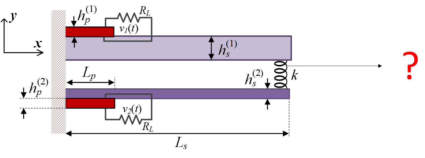
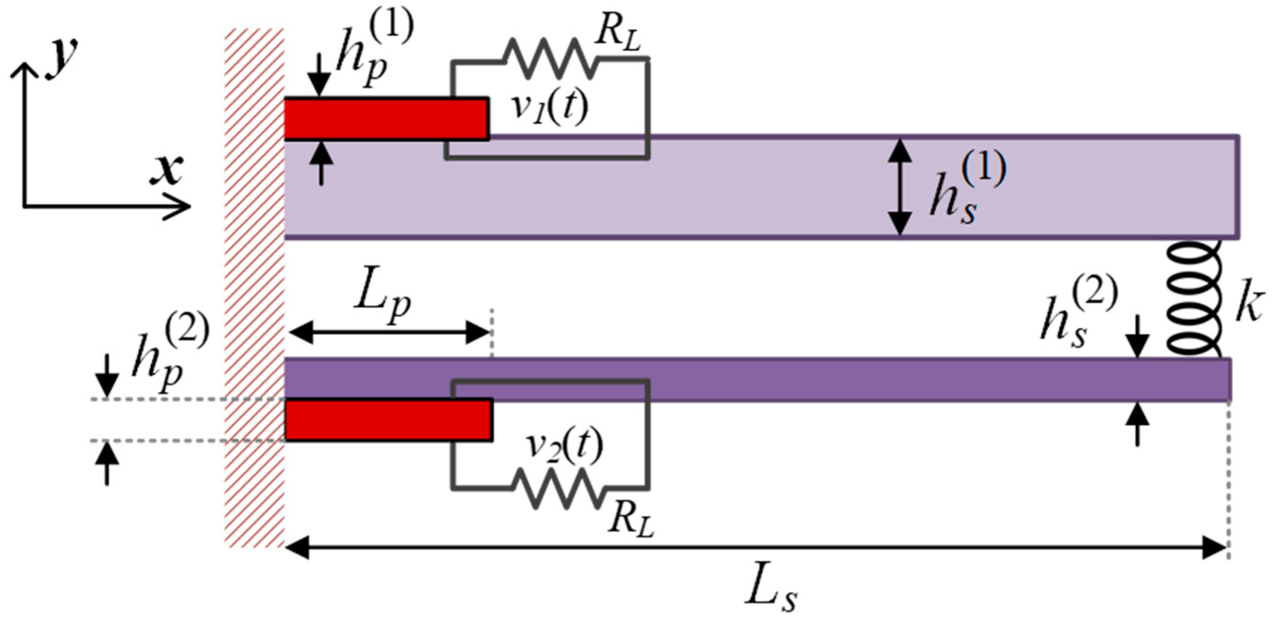
Figure 1 shows that the lengths of both piezoelectric patches are very small compared to the length of the beams. As a result, they have negligible effects on the mode shapes. Therefore, in the upcoming derivations (which aim to find the mode shapes of the coupled system) the effects of the piezoelectric patches are ignored.

By utilizing Hamilton’s principal, the normalized free vibration equations of the system and the corresponding kinematic and natural boundary conditions are derived as [21].

Equations of motion:

$$\frac{{\partial }^4{w}_1\left(x,t\right)}{\partial x^4}+\frac{{\partial }^2{w}_1\left(x,t\right)}{\partial t^2}=0$$

(1)

$$\frac{{\partial }^4{w}_2\left(x,t\right)}{\partial x^4}+\left(\frac{A_s^{\left(2\right)}{I}_s^{\left(1\right)}}{A_s^{\left(1\right)}{I}_s^{\left(2\right)}}\right)\frac{{\partial }^2{w}_2\left(x,t\right)}{\partial t^2}=0$$

(2)

Kinematic boundary conditions:

$$w_1\left(0,t\right)=w_2\left(0,t\right)={\frac{\partial w_1}{\partial x}|}_{\left(0,t\right)}={\frac{\partial w_2}{\partial x}|}_{\left(0,t\right)}=0$$

(3)

Natural boundary conditions:

$${\frac{{\partial }^2{w}_1}{\partial x^2}|}_{\left(1,t\right)}={\frac{{\partial }^2{w}_2}{\partial x^2}|}_{\left(1,t\right)}=0$$

(4)

$$w_1\left(1,t\right)-w_2\left(1,t\right)+{\left(-1\right)}^i\left(\frac{E_s{I}_s^{\left(i\right)}}{k{L}_s^3}\right){\frac{{\partial }^3{w}_i}{\partial x^3}|}_{\left(1,t\right)}=0,i=1,2$$

(5)

In these equations $L_s$, is the length of the beams, $E_s$ is the Young’s modulus of the beams material, $I_s^{\left(i\right)}$, $i=1,2$ represents the second area moment of inertia of the $i$th beam’s cross section around its neutral axis, $A_s^{\left(i\right)}$ is the area cross section of the $i$th beam and $k$ is the elastic constant of the connecting linear spring. Moreover, the normalized variables $x$, $w_i$ and $t$ are defined by

$$x=\frac{\widehat{x}}{L_s},w_i=\frac{{\widehat{w}}_i}{L_s},t=\frac{\widehat{t}}{T}$$

(6)

where ${\widehat{w}}_i$ is the deflection of the $i$th beam and $T=L_s^2\sqrt{{\rho }_s{A}_s^{\left(1\right)}/E_s{I}_s^{\left(1\right)}}$ in which ${\rho }_s$ is the material density.

The dynamic response of a linear continuous system can be expressed as a linear combination of its mode shapes [21]. Therefore, an essential first step in the dynamic modelling of a continuous structure, either single or multi-body, is to find the mode shapes of that system. A mode shape of a system is a state of motion of that system in which all of its elements move with the same frequency and phase, but not necessarily with the same amplitude. Appendix A presents the derivation of the exact natural frequencies and the mode shapes of the system. To verify the accuracy of the proposed analytical technique, a system with physical and geometrical parameters given in

Table 1. Physical and geometrical parameter values of the system.

Parameter	Symbol	Unit	Value
Length of the beam	$L_s$	mm	305
Thickness of the thick beam	$h_s^{\left(1\right)}$	mm	0.5
Thickness of the thin beam	$h_s^{\left(2\right)}$	mm	0.25
Width of the beams	$b_s$	mm	16
Young’s modulus	$E_s$	GPa	210
Mass density of beams	${\rho }_s$	kg/m3	7000

is considered.

Using the numerical values reported in Table 1, the first three normalized natural frequencies of the system are obtained as given in

Table 2. The first three natural frequencies of the system.

Mode Number	Analytical (rad/s)	FEA (rad/s)	Error (%)
1	25.6611	25.6610	$0.0001$
2	71.7585	71.7585	$0.0000$
3	167.1232	167.1232	$0.0000$

. In this table, the analytical results are compared with those of finite element (FE) simulations using the commercial software Abaqus. The numerical and analytical results are in excellent agreement.

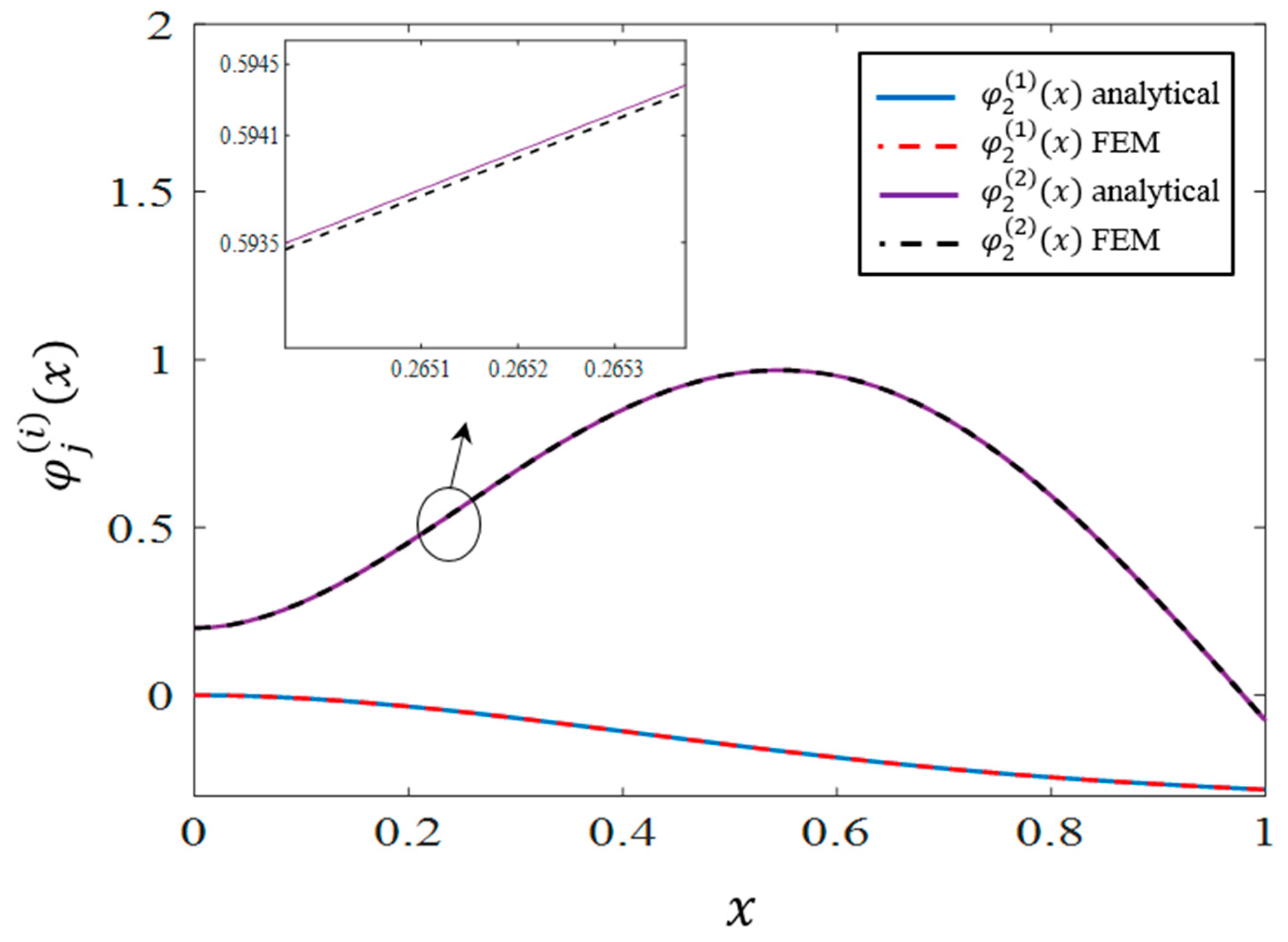
In order to investigate the accuracy of the analytical mode shapes, Figure 2, Figure 3 and Figure 4 are provided. In these figures, the first three analytical and FE modes are compared, and acceptable agreement is observed. To make the numerical and analytic modes comparable, they have both been normalized such that ${{\displaystyle \int }}_0^1{\left({\phi }_i^{\left(1\right)}\left(x\right)\right)}^{2}dx+\left(\frac{A_2{I}_1}{A_1{I}_2}\right){{\displaystyle \int }}_0^1{\left({\phi }_i^{\left(2\right)}\left(x\right)\right)}^{2}dx=1$.

2.2. Dynamic Analysis

Lagrange’s equations are employed here to derive the differential equations governing the dynamic behavior of the system. This requires the analytical expressions for the potential and kinetic energies, as well as the virtual work done on the system. The potential energy of the system shown in Figure 1 is composed of three parts: (1) strain energy of the substructure, ${\pi }_s$, (2) potential energy of the piezoelectric material, ${\pi }_p$, and (3) strain energy of the spring, ${\pi }_e$.

• Strain Energy of the Substructure

Assuming linear elastic material for the beams, the strain energy of the harvester can be written as

$${\widehat{\pi }}_s=\frac{1}{2}{E}_s{\displaystyle \sum }_{k=1}^2({I^{\prime }}_s^{\left(k\right)}{{\displaystyle \int }}_o^{L_p}{\left(\frac{{\partial }^2{\widehat{w}}_k\left(\widehat{x},\widehat{t}\right)}{\partial {\widehat{x}}^2}\right)}^{2}d\widehat{x}+I_s^{\left(k\right)}{{\displaystyle \int }}_{L_p}^{L_s}{\left(\frac{{\partial }^2{\widehat{w}}_k\left(\widehat{x},\widehat{t}\right)}{\partial {\widehat{x}}^2}\right)}^{2}d\widehat{x})$$

(7)

where $L_p$ the length of the piezoelectric patches (see Appendix B) and

$$I_s^{\left(k\right)}=b_s{{\displaystyle \int }}_{-\frac{h_s^{\left(k\right)}}{2}}^{\frac{h_s^{\left(k\right)}}{2}}{\widehat{y}}^{2}d\widehat{y}=\frac{1}{12}{b}_s{\left(h_s^{\left(k\right)}\right)}^3$$

(8)

$${I^{\prime }}_s^{\left(k\right)}=b_s{{\displaystyle \int }}_{-h_{sa}^{\left(k\right)}}^{h_{pa}^{\left(k\right)}-h_p}{\widehat{y}}^{2}d\widehat{y}=\frac{b_s}{3}\left({\left(h_{pa}^{\left(k\right)}-h_p\right)}^3+{\left(h_{sa}^{\left(k\right)}\right)}^3\right)$$

(9)

• Potential Energy of the Piezoelectric Layers

The potential energy of the piezoelectric material, ${\widehat{\pi }}_p$, is composed of a strain energy ${\widehat{U}}_p$ and a potential electrical component ${\widehat{W}}_{ie}$. The strain energy of the piezoelectric layers in the system shown in Figure 1 can be expressed as [22]

$${\widehat{U}}_p=\frac{1}{2}{\displaystyle \sum }_{k=1}^2{{\displaystyle \int }}^{ }{\sigma }_p^{\left(k\right)}{\epsilon }_p^{\left(k\right)}d{\forall }_p^{\left(k\right)}$$

(10)

where ${\sigma }_p^{\left(1\right)}$ and ${\sigma }_p^{\left(2\right)}$ are respectively the normal stress components of the piezoelectric layers attached to the thick and thin beams, while ${\epsilon }_p^{\left(1\right)}$ and ${\epsilon }_p^{\left(2\right)}$ are their strain counterparts. Moreover, ${\forall }_p^{\left(k\right)}$ is the volume of the kth piezoelectric layer. The following constitutive equations show the relation between the stress and strain in the piezoelectric layers [23]:

$${\sigma }_p^{\left(j\right)}=E_p{\epsilon }_p^{\left(j\right)}-e_{31}{E}_3^{\left(j\right)}, j=1,2$$

(11)

$$D_3^{\left(j\right)}=e_{31}{\epsilon }_p^{\left(j\right)}+{\epsilon }_{33}^p{E}_3^{\left(j\right)}, j=1,2$$

(12)

In Equations (11) and (12), $D_3^{\left(i\right)}$ and $E_3^{\left(i\right)}$ denote the vector of electrical displacement and the electric field of the ith piezoelectric material in $\widehat{y}$ direction, $e_{31}$ represents the piezoelectric stress coefficient, and ${\epsilon }_{33}^{\left(p\right)}$ is the dielectric constant of the piezoelectric material. In addition, as explained earlier, $E_p$ is the elastic modulus of the piezoelectric layer.

Substituting Equation (11) into (10), assuming $E_3^{\left(k\right)}\left(t\right)=-{\widehat{v}}_k\left(t\right)/h_p$ [24] (where ${\widehat{v}}_k\left(t\right)$ is the generated voltage in the kth piezo layer) and employing the stress–strain relationships, one may simplify the ${\widehat{U}}_p$ expression as

$$\begin{array}{ll}{\widehat{U}}_p& =\frac{1}{2}{E}_p{I}_p^{\left(k\right)}{\displaystyle {\displaystyle \sum }_{k=1}^2}{{\displaystyle \int }}_o^{L_p}{\left(\frac{{\partial }^2{\widehat{w}}_k\left(\widehat{x},\widehat{t}\right)}{\partial {\widehat{x}}^2}\right)}^{2}d\widehat{x}\\ & -{\displaystyle {\displaystyle \sum }_{k=1}^2}\left(\frac{e_{31}{z}_p^{\left(k\right)}}{2h_p}{{\displaystyle \int }}_o^{L_p}\frac{{\partial }^2{\widehat{w}}_k\left(\widehat{x},\widehat{t}\right)}{\partial {\widehat{x}}^2}d\widehat{x}\right){\widehat{v}}_k\left(\widehat{t}\right)\end{array}$$

(13)

where $I_p^{\left(k\right)}$ and $z_p^{\left(k\right)}$ are defined as

$$I_p^{\left(k\right)}=b_p{{\displaystyle \int }}_{h_{pa}^{\left(k\right)}-h_p}^{h_{pa}^{\left(k\right)}}{\widehat{y}}^{2}d\widehat{y}=\frac{b_p}{3}\left({\left(h_{pa}^{\left(k\right)}\right)}^3-{\left(h_{pa}^{\left(k\right)}-h_p\right)}^3\right)$$

(14)

$$z_p^{\left(k\right)}=b_p{{\displaystyle \int }}_{h_{pa}^{\left(k\right)}-h_p}^{h_{pa}^{\left(k\right)}}\widehat{y}d\widehat{y}=\frac{b_p}{2}\left({\left(h_{pa}^{\left(k\right)}\right)}^2-{\left(h_{pa}^{\left(k\right)}-h_p\right)}^2\right)$$

(15)

The internal electrical energy generated in the piezoelectric layers, ${\widehat{W}}_{ie}$, can be expressed as [23]

$${\widehat{W}}_{ie}=\frac{1}{2}{\displaystyle \sum }_{k=1}^2{{\displaystyle \int }}_{{\forall }_p^{\left(k\right)}}{E}_3^{\left(k\right)}{D}_3^{\left(k\right)}d{\forall }_p^{\left(k\right)}$$

(16)

By substituting $D_3^{\left(k\right)}$ from Equation (12), considering $E_3^{\left(k\right)}=-{\widehat{v}}_k\left(t\right)/h_p$ and employing the strain-displacement relation ${\widehat{\mathsf{\epsilon }}}_{\mathrm{p}}^{\left(\mathrm{k}\right)}=-\mathrm{y}{\partial }^2\widehat{\mathrm{w}}/\partial {\widehat{\mathrm{x}}}^2$, Equation (16) can be simplified in terms of ${\widehat{w}}_1$ and ${\widehat{w}}_2$ as

$${\widehat{W}}_{ie}\left(t\right)=-\frac{1}{2}{\displaystyle \sum }_{k=1}^2\left(\left(J_p^{\left(k\right)}{{\displaystyle \int }}_0^{L_p}\frac{{\partial }^2{\widehat{w}}_k\left(\widehat{x},\widehat{t}\right)}{\partial {\widehat{x}}^2}d\widehat{x}\right){\widehat{v}}_k\left(t\right)-c_{\rho }^{\left(k\right)}{\widehat{v}}_k^2\left(t\right)\right)$$

(17)

in which

$$c_{\rho }^{\left(k\right)}={\epsilon }_{33}^p\frac{A_p^{\left(k\right)}}{h_p}$$

(18)

$$J_p^{\left(k\right)}=\frac{e_{31}}{h_p}{{\displaystyle \int }}_{h_{pa}^{\left(k\right)}-h_p}^{h_{pa}^{\left(k\right)}}\widehat{y}{b}_{p}d\widehat{y}=\frac{e_{31}{b}_p}{2h_p}\left({\left(h_{pa}^{\left(k\right)}\right)}^2-{\left(h_{pa}^{\left(k\right)}-h_p\right)}^2\right)$$

(19)

Thus, the total potential energy of piezoelectric layers is obtained as

$${\widehat{\pi }}_p={\widehat{U}}_p-{\widehat{W}}_{ie}$$

(20)

• Strain Energy of the Connecting Spring

The elastic strain energy of the linear connecting spring, ${\widehat{\pi }}_e$, is simply

$${\widehat{\pi }}_e=\frac{1}{2}k{\left({\widehat{w}}_1\left(L_s,\widehat{t}\right)-{\widehat{w}}_2\left(L_s,\widehat{t}\right)\right)}^2$$

(21)

Assuming that the mass of the spring is negligible, the kinetic energy of the system can be derived by adding the kinetic energies of the constitutive beams and the piezoelectric layers as

$$\begin{array}{ll}\widehat{{\rm K}}& =\frac{1}{2}{\rho }_s{A}_s^{\left(k\right)}{\displaystyle {\displaystyle \sum }_{k=1}^2}{{\displaystyle \int }}_0^{L_s}{\left(\frac{d\widehat{Y}\left(\widehat{t}\right)}{d\widehat{t}}+\frac{\partial {\widehat{w}}_k\left(\widehat{x},\widehat{t}\right)}{\partial \widehat{t}}\right)}^{2}d\widehat{x}\\ & +\frac{1}{2}{\rho }_p{A}_p^{\left(k\right)}{\displaystyle {\displaystyle \sum }_{k=1}^2}{{\displaystyle \int }}_0^{L_p}{\left(\frac{d\widehat{Y}\left(\widehat{t}\right)}{d\widehat{t}}+\frac{\partial {\widehat{w}}_k\left(\widehat{x},\widehat{t}\right)}{\partial \widehat{t}}\right)}^{2}d\widehat{x}\end{array}$$

(22)

where $\widehat{Y}$ is the base displacement.

To account for the modal damping, it is assumed that the system is vibrating in a linearly damped viscous media. The damping coefficient for both beams is assumed to be $c$ per unit length. In such a condition, the virtual work done on the system due to this damping will be as

$$\delta {\widehat{W}}_{ext}^{\left(c\right)}=-c{\displaystyle \sum }_{k=1}^2{{\displaystyle \int }}_0^{L_s}\frac{\partial {\widehat{w}}_k\left(\widehat{x},\widehat{t}\right)}{\partial \widehat{t}}\delta {\widehat{w}}_k\left(\widehat{x},\widehat{t}\right)d\widehat{x}$$

(23)

In addition, as the electrical charge is $Q_i$, $i=1,2$, in the load circuit with resistance $R_l^{\left(i\right)}$, the virtual work is

$$\delta {\widehat{W}}_{ext}^{\left(R_l\right)}\left(\widehat{t}\right)=Q_1\left(\widehat{t}\right)\delta {\widehat{v}}_1\left(\widehat{t}\right)+Q_2\left(\widehat{t}\right)\delta {\widehat{v}}_2\left(\widehat{t}\right)$$

(24)

Hence, the effective virtual work done to the system can be summarized as

$$\begin{array}{ll}\delta {\widehat{W}}_{ext}\left(\widehat{t}\right)& =\delta {\widehat{W}}_{ext}^{\left(R_l\right)}\left(\widehat{t}\right)+\delta {\widehat{W}}_{ext}^{\left(c\right)}\left(\widehat{t}\right)=Q_1\left(\widehat{t}\right)\delta {\widehat{v}}_1\left(\widehat{t}\right)+Q_2\left(\widehat{t}\right)\delta {\widehat{v}}_2\left(\widehat{t}\right)\\ & -c{\displaystyle {\displaystyle \sum }_{k=1}^2}{{\displaystyle \int }}_0^{L_s}\frac{\partial {\widehat{w}}_k\left(\widehat{x},\widehat{t}\right)}{\partial \widehat{t}}\delta {\widehat{w}}_k\left(\widehat{x},\widehat{t}\right)d\widehat{x}\end{array}$$

(25)

The dynamic response of linear systems can be effectively approximated as a linear combination of their mode shapes. This theory has been examined and verified in many published studies [5,25]. Hence, for the system under study,

$${\widehat{w}}_k\left(\widehat{x},\widehat{t}\right)={\displaystyle \sum }_{i=1}^n{\widehat{\phi }}_i^{\left(k\right)}\left(\widehat{x}\right){\widehat{q}}_i\left(\widehat{t}\right), k=1,2$$

(26)

where ${\widehat{q}}_i$ represents the contribution of the $i$th mode in the dynamic response. Now, ${\widehat{q}}_i$, as well as ${\widehat{v}}_1$ and ${\widehat{v}}_2$, can be considered as the generalized coordinates. By substituting Equation (26) into (7), (20), (21), (22), and (25), while employing Lagrange’s equation, after some simple manipulations, the governing equations are derived. For notational simplicity, the following normalized variable is defined

$$v_i=\frac{{\widehat{v}}_i}{\mathbb{V}}, i=1,2$$

(27)

where $\mathbb{V}$ is defined as $\mathbb{V}=\frac{h_p{d}_{31}{E}_p{h}_{pc}^{\left(1\right)}}{{\epsilon }_{33}^s{L}_p}$. Further, the parameter $h_{pc}^{\left(k\right)}$ is the distance between the center of the piezoelectric layer and the neutral axis and $d_{31}$ and ${\epsilon }_{33}^s$ are piezoelectric constants whose typical values are given in

Table 3. Physical and geometrical properties of the piezoelectric materials.

Parameter	Symbol	Unit	Value
Width of the piezoelectric layers	$b_p$	mm	7
Young’s modulus of the piezoelectric layer	$E_p$	GPa	66
Permittivity	${\epsilon }_{33}^s$	nF/m	15.93
Piezoelectric constant	$d_{31}$	pm/v	−190
Mass density of the piezoelectric layer	${\rho }_p$	kg/m3	7800
Electrical resistance	$R_l$	$\mathrm{M}\Omega$	0.2
Thickness of the piezoelectric layers	$h_p$	mm	0.25

. Using the normalized variable $q=\widehat{q}/L_s$, the dimensionless governing equations are reduced to

$$\begin{array}{ll}{\left[M\right]}_{n\times n}{\ddot{\overrightarrow{q}}}_{n\times 1}\left(t\right)& +{\left[C\right]}_{n\times n}{\dot{\overrightarrow{q}}}_{n\times 1}\left(t\right)+{\left[K\right]}_{n\times n}{\overrightarrow{q}}_{n\times 1}\left(t\right)\\ & =\ddot{Y}\left(t\right)\times \overrightarrow{f}+{\displaystyle {\displaystyle \sum }_{k=1}^2}{\overrightarrow{\Omega }}_{n\times 1}^{\left(k\right)}{v}_k\left(t\right)\end{array}$$

(28)

$${\dot{v}}_k\left(t\right)+\zeta v_k\left(t\right)+{\vartheta }_k{\displaystyle \sum }_{i=1}^n\left({{\displaystyle \int }}_0^{\frac{L_p}{L_s}}\frac{d^2{\phi }_i^{\left(k\right)}}{d{x}^2}dx\right)\frac{d{q}_i\left(t\right)}{dt}=0, k=1,2$$

(29)

In Equation (29), $\zeta$ and ${\vartheta }_k$ are defined as

$$\zeta =\frac{T{h}_p}{R_l{\epsilon }_{33}^s{b}_p{L}_p}, {\vartheta }_1=1, {\vartheta }_2=\frac{h_{pc}^{\left(2\right)}}{h_{pc}^{\left(1\right)}}$$

(30)

In these equations, $\dot{( )}$ represents differentiation with respect to normalized time $t$. Moreover, the elements of the matrices ${\left[M\right]}_{n\times n}$, ${\left[C\right]}_{n\times n}$, ${\left[K\right]}_{n\times n}$ and vectors ${\overrightarrow{f}}_{n\times 1}$ and ${\overrightarrow{\mathsf{\Omega }}}_{n\times 1}^{\left(k\right)}$ are functions of the mode shapes as well as the physical and geometrical parameters of the system, and are given by

$$\begin{array}{ll}{M}_{ij}{M}_{ij}& =\frac{L_s{}^3}{T^2}\left({\rho }_s{\displaystyle {\displaystyle \sum }_{k=1}^2}{A}_s^{\left(k\right)}{{\displaystyle \int }}_0^1{\phi }_i^{\left(k\right)}\left(x\right){\phi }_j^{\left(k\right)}\left(x\right)dx\right)\\ & =\frac{L_s{}^3}{T^2}\left({\rho }_s{\displaystyle {\displaystyle \sum }_{k=1}^2}{A}_s^{\left(k\right)}{{\displaystyle \int }}_0^1{\phi }_i^{\left(k\right)}\left(x\right){\phi }_j^{\left(k\right)}\left(x\right)dx\right)+\end{array}$$

(31)

$$C_{ij}=c\frac{L_s^4}{T}\left({\displaystyle \sum }_{k=1}^2{{\displaystyle \int }}_0^1{\phi }_i^{\left(k\right)}\left(x\right){\phi }_j^{\left(k\right)}\left(x\right)dx\right)$$

(32)

$$\begin{array}{ll}{K}_{ij}& =\frac{E_p}{L_s}\left({\displaystyle {\displaystyle \sum }_{k=1}^2}{I}_p^{\left(k\right)}{{\displaystyle \int }}_0^{\frac{L_p}{L_s}}\frac{d^2{\phi }_i^{\left(k\right)}\left(x\right)}{d{x}^2}\frac{d^2{\phi }_j^{\left(k\right)}\left(x\right)}{d{x}^2}dx\right)\\ & +\frac{E_s}{L_s}\left({\displaystyle {\displaystyle \sum }_{k=1}^2}{I^{\prime }}_s^{\left(k\right)}{{\displaystyle \int }}_0^{\frac{L_p}{L_s}}\frac{d^2{\phi }_i^{\left(k\right)}\left(x\right)}{d{x}^2}\frac{d^2{\phi }_j^{\left(k\right)}\left(x\right)}{d{x}^2}dx\right)\\ & +\frac{E_s}{L_s}\left({\displaystyle {\displaystyle \sum }_{k=1}^2}{I}_s^{\left(k\right)}{{\displaystyle \int }}_{\frac{L_p}{L_s}}^1\frac{d^2{\phi }_i^{\left(k\right)}\left(x\right)}{d{x}^2}\frac{d^2{\phi }_j^{\left(k\right)}\left(x\right)}{d{x}^2}dx\right)\end{array}$$

(33)

$$f_i=-\frac{L_s{}^3}{T^2}\left({\rho }_s{\displaystyle \sum }_{k=1}^2{A}_s^{\left(k\right)}{{\displaystyle \int }}_0^1{\phi }_i^{\left(k\right)}\left(x\right)dx+{\rho }_p{\displaystyle \sum }_{k=1}^2{A}_p{{\displaystyle \int }}_0^{\frac{L_p}{L_s}}{\phi }_i^{\left(k\right)}\left(x\right)dx\right)$$

(34)

$${\Omega }_i^{\left(k\right)}\left(t\right)={\gamma }^{\left(k\right)}{{\displaystyle \int }}_0^{\frac{L_p}{L_s}}\left(\frac{d^2{\phi }_i^{\left(k\right)}\left(x\right)}{d{x}^2}\right)dx$$

(35)

where ${\gamma }^{\left(k\right)}$ in Equation (35) is calculated as

$${\gamma }^{\left(k\right)}=\mathbb{V}\left(-\frac{1}{2}{J}_p^{\left(k\right)}-\frac{e_{31}}{2h_p}{I^{\prime }}_p^{\left(k\right)}\right)$$

(36)

In addition, ${I^{\prime }}_p^{\left(k\right)}$ in Equation (36) is

$${I^{\prime }}_p^{\left(k\right)}=\frac{1}{2}{b}_p\left({\left(h_{pa}^{\left(k\right)}-h_p\right)}^2-{\left(h_{pa}^{\left(k\right)}\right)}^2\right), k=1,2$$

(37)

In the next step, the dynamic Equations (28) and (29) are transformed into state space. To do so, the state vector $\overrightarrow{P}$ is defined as

$$\overrightarrow{P}={\left[q_1 q_2\dots q_n⋮{\dot{q}}_1 {\dot{q}}_2\dots {\dot{q}}_n⋮ v_1 v_2\right]}^{\mathbb{T}}$$

(38)

where the superscript $\mathbb{T}$ denotes the transpose operator. The state space equations governing the dynamic behavior of the system are then

$$\dot{\overrightarrow{P}}\left(t\right)=\left[A\right]\overrightarrow{P}\left(t\right)+\left[B\right]\ddot{Y}\left(t\right)$$

(39)

In Equation (39), the matrices $\left[A\right]$ and $\left[B\right]$ are defined as

$$\left[A\right]=\left[\begin{array}{ccc}{\left[0\right]}_{n\times n}& {\left[I\right]}_{n\times n}& {\left[0\right]}_{n\times 2}\\ -{\left[M\right]}^{-1}\left[K\right]& -{\left[M\right]}^{-1}\left[C\right]& {\left[M\right]}^{-1}\left[{\Omega }_1^{\left(k\right)} {\Omega }_2^{\left(k\right)} \right]\\ {\left[0\right]}_{2\times n}& {\left[D\right]}_{2\times n}& -\zeta {\left[I\right]}_{2\times 2}\end{array}\right], \left[B\right]=\left\{\begin{array}{c}{\left[0\right]}_{n\times 1}\\ {\left[M\right]}^{-1}\overrightarrow{f}\\ {\left[0\right]}_{2\times 1}\end{array}\right\}$$

(40)

The matrix $\left[D\right]$ in Equation (40) is defined as

$${\left[D\right]}_{i,j}={\mu }_i{{\displaystyle \int }}_0^{\frac{L_p}{L_s}}\frac{d^2{\phi }_j^{\left(i\right)}}{d{x}^2}dx$$

(41)

where ${\mu }_1=\mathbb{V}$ and ${\mu }_2=\mathbb{V}{\vartheta }_2$.

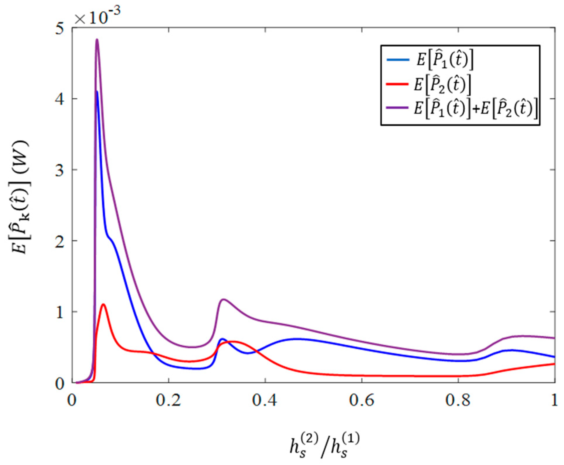
To investigate the number of modes that contribute significantly to the dynamic response, a physical system with the specifications given in Table 1 (for the substructure) and Table 3 (for the piezoelectric materials) is considered. Moreover, here and in the rest of this paper, unless otherwise stated, the damping $c$ is selected such that the modal damping of the first mode becomes a nominal value of 0.01.

2.3. Validation

To further investigate the accuracy of the presented formulation, the natural frequencies of the harvester are compared with those presented in [26]. To this end, a harvester with zero coupling and mechanical properties as stated in

Table 4. Physical and geometrical parameter values of the sample structure.

Parameter	Symbol	Unit	Value
Length of the beam	$L_s$	mm	100
Thickness of the thick beam	$h_s^{\left(1\right)}$	mm	0.5
Thickness of the thin beam	$h_s^{\left(2\right)}$	mm	0. 5
Width of the beams	$b_s$	mm	20
Young’s modulus of the beams	$E_s$	GPa	100
Mass density of beams	${\rho }_s$	kg/m3	7165

and

Table 5. Physical and geometrical properties of the sample piezoelectric materials.

Parameter	Symbol	Unit	Value
Width of the piezoelectric layers	$b_p$	mm	20
Young’s modulus of the piezoelectric layer	$E_p$	GPa	66
Permittivity	${\epsilon }_{33}^s$	nF/m	15.93
Piezoelectric constant	$d_{31}$	pm/v	−190
Mass density of the piezoelectric layer	${\rho }_p$	kg/m3	7800

is considered.

The frequency response curves for the sample harvester, resulting from the base acceleration for $R_l=1 \mathrm{M}\Omega$ (see

Table 6. Comparison between the natural frequencies when $R_l=100 \Omega$.

Natural Frequency	Present Study (Hz)	Ref. [26] (Hz)	Error (%)
First Mode	48.06	47.8	$0.543$
Second Mode	299.7	299.6	$0.033$
Third mode	838.9	838.2	$0.083$

) and $R_l=100 \Omega$ (see

Table 7. Comparison between the natural frequencies when $R_l=1 \mathrm{M}\Omega$.

Natural Frequency	Present Study (Hz)	Ref. [26] (Hz)	Error (%)
First Mode	48.83	48.8	$0.0614$
Second Mode	301.4	301.5	$-0.031$
Third mode	840.9	839.2	$0.202$

), are illustrated in Figure 5. The exact values of the natural frequencies in which the voltage response peaks, are compared with the results presented in [26]. Regarding the peak and error values presented in the tables, it is evident that the present model acceptably predicts the resulting voltage from the harvester.

3. Random Vibration Analysis

A necessary first step in the random vibration analysis of a dynamic system is to obtain the frequency response functions. The frequency response matrix $\left[H_P^{\left(\ddot{Y}\right)}\left(\omega \right)\right]$. of the linear system (Equation (39)), can be derived as

$${\left[H_P^{\left(\ddot{Y}\right)}\left(\omega \right)\right]}_{\left(2n+2\right)\times 1}={\left(j^{*}\omega {\left[I\right]}_{\left(2n+2\right)\times \left(2n+2\right)}-{\left[A\right]}_{\left(2n+2\right)\times \left(2n+2\right)}\right)}^{-1}{\left[B\right]}_{\left(2n+2\right)\times 1}$$

(42)

The mathematical details to obtain Equation (42) are given in Appendix C and $j^{*}=\sqrt{-1}$. The frequency response function corresponding to $w_k\left(x,t\right)$ can also be easily derived by substituting $w_k\left(x,t\right)=H_{w_k}^{\left(\ddot{Y}\right)}\left(x,\omega \right){\ddot{Y}}_0\exp (j^{*}\omega t)$ and $q_i\left(t\right)=H_{P_i}^{\left(\ddot{Y}\right)}\left(\omega \right){\ddot{Y}}_0\exp (j^{*}\omega t)$ (with ${\overrightarrow{H}}_{P_i}^{\left(\ddot{Y}\right)}\left(\omega \right)$ being the $i$th element of the frequency response matrix derived in Equation (42)) into the normalized form of Equation (26) and cancelling $\exp \left(j^{*}\omega t\right)$ from both sides. Consequently, one can get

$$H_{w_k}^{\left(\ddot{Y}\right)}\left(x,\omega \right)={\displaystyle \sum }_{i=1}^n{\phi }_i^{\left(k\right)}\left(x\right){\overrightarrow{H}}_{P_i}^{\left(\ddot{Y}\right)}\left(\omega \right)$$

(43)

Figure 6 shows the magnitude of the frequency response functions of the normalized tip displacements $w_1\left(1,t\right)$ and $w_2\left(1,t\right)$ of the undamped system. The frequency responses of the generated voltages are also illustrated in Figure 7. These frequency responses will be used later to derive the statistical properties of the harvested power.

The frequency response functions are closely related to the impulse response functions. The impulse response of the system is the consequent dynamics $\overrightarrow{P}\left(t\right)=\overrightarrow{h}\left(t\right)$, corresponding to the application of a unit impulse input $\ddot{Y}\left(t\right)=\delta \left(t\right)$. Using Laplace transform, this impulse response function can be easily derived as

$$\overrightarrow{P}\left(t\right)=\overrightarrow{h}\left(t\right)={ℒ}^{-1}\left[{\left(s\left[I\right]-\left[A\right]\right)}^{-1}B\right]$$

(44)

The following equation characterizes the relationship of the frequency and impulse response functions [15]

$$\overrightarrow{H}\left(\omega \right)={{\displaystyle \int }}_{-\infty }^{+\infty }\overrightarrow{h}\left(\theta \right)\exp \left(-j^{*}\omega \theta \right)d\theta$$

(45)

Having established the impulse response function, the dynamic response of the system to a general input $\ddot{Y}\left(t\right)$ can be obtained using the following convolution integral [15].

$$\overrightarrow{P}\left(t\right)={{\displaystyle \int }}_{-\infty }^{+\infty }\overrightarrow{h}\left(\theta \right)\ddot{Y}\left(t-\theta \right)d\theta$$

(46)

Using Equation (46), the cross-correlation function $R_{p_i{p}_j}\left(\tau \right)$ is calculated as

$$\begin{array}{ll}{R}_{p_i{p}_j}\left(\tau \right)& =E\left[{{\displaystyle \int }}_{-\infty }^{+\infty }{h}_i\left({\theta }_1\right)\ddot{Y}\left(t-{\theta }_1\right)d{\theta }_1{{\displaystyle \int }}_{-\infty }^{+\infty }{h}_j\left({\theta }_2\right)\ddot{Y}\left(t+\tau -{\theta }_2\right)d{\theta }_2\right]\\ & =E\left[{{\displaystyle \int }}_{-\infty }^{+\infty }{{\displaystyle \int }}_{-\infty }^{+\infty }{h}_i\left({\theta }_1\right)h_j\left({\theta }_2\right)\ddot{Y}\left(t-{\theta }_1\right)\ddot{Y}\left(t+\tau -{\theta }_2\right)d{\theta }_{1}d{\theta }_2\right]\end{array}$$

(47)

Assuming a stationary process for $\ddot{Y}\left(t\right)$, Equation (47) can be further simplified as

$$R_{p_i{p}_j}\left(\tau \right)={{\displaystyle \int }}_{-\infty }^{+\infty }{{\displaystyle \int }}_{-\infty }^{+\infty }{h}_i\left({\theta }_1\right)h_j\left({\theta }_2\right)R_{\ddot{Y}}\left(\tau -{\theta }_2+{\theta }_1\right)d{\theta }_{1}d{\theta }_2$$

(48)

in which $R_{\ddot{Y}}\left(\tau +{\theta }_1-{\theta }_2\right)$ is the autocorrelation function of $\ddot{Y}\left(t\right)$.

By choosing $i=j$ in Equation (48), the autocorrelation function $R_{p_i}\left(\tau \right)$ is obtained as

$$R_{p_i}\left(\tau \right)={{\displaystyle \int }}_{-\infty }^{+\infty }{{\displaystyle \int }}_{-\infty }^{+\infty }{h}_i\left({\theta }_1\right)h_i\left({\theta }_2\right)R_{\ddot{Y}}\left(\tau -{\theta }_2+{\theta }_1\right)d{\theta }_{1}d{\theta }_2$$

(49)

Having a closed form relation for $R_{p_i{p}_j}\left(x,\tau \right)$, the autocorrelation function for $w_k\left(x,t\right)$ can also be derived as

$$R_{w_k}\left(x,\tau \right)=E\left[\left({\displaystyle \sum }_{i=1}^n{\phi }_i^{\left(k\right)}\left(x\right)p_i\left(t\right)\right)\left({\displaystyle \sum }_{j=1}^n{\phi }_j^{\left(k\right)}\left(x\right)p_j\left(t+\tau \right)\right)\right]$$

(50)

Upon simplification, $R_{w_k}\left(x,\tau \right)$ can be expressed as

$$\begin{array}{ll}{R}_{w_k}\left(x,\tau \right)& =E\left[{\displaystyle {\displaystyle \sum }_{j=1}^n}{\displaystyle {\displaystyle \sum }_{i=1}^n}{\phi }_i^{\left(k\right)}\left(x\right){\phi }_j^{\left(k\right)}\left(x\right)p_i\left(t\right)p_j\left(t+\tau \right)\right]\\ & =\left({\displaystyle {\displaystyle \sum }_{j=1}^n}{\displaystyle {\displaystyle \sum }_{i=1}^n}{\phi }_i^{\left(k\right)}\left(x\right){\phi }_j^{\left(k\right)}\left(x\right)E\left[p_i\left(t\right)p_j\left(t+\tau \right)\right]\right) \\ & =\left({\displaystyle {\displaystyle \sum }_{i=1}^n}{\displaystyle {\displaystyle \sum }_{i=1}^n}{\phi }_i^{\left(k\right)}\left(x\right){\phi }_j^{\left(k\right)}\left(x\right)R_{p_i{p}_j}\left(\tau \right)\right)\end{array}$$

(51)

The cross spectral density of $p_i$ and $p_j$ is defined as $s_{p_i{p}_j}\left(\omega \right)=1/2\pi {{\displaystyle \int }}_{-\infty }^{\infty }{R}_{p_i{p}_j}\left(\tau \right)\exp \left(-j\omega \tau \right)d\tau$. By substituting Equation (48) into this equation, one gets

$$S_{p_i{p}_j}\left(\omega \right)=\frac{1}{2\pi }{{\displaystyle \int }}_{-\infty }^{+\infty }{{\displaystyle \int }}_{-\infty }^{+\infty }{{\displaystyle \int }}_{-\infty }^{+\infty }{h}_i\left({\theta }_1\right)h_j\left({\theta }_2\right)R_{\ddot{Y}}\left(\tau -{\theta }_2+{\theta }_1\right)\exp \left(-j\omega \tau \right)d{\theta }_{1}d{\theta }_{2}d\tau$$

(52)

By defining $\gamma =\tau -{\theta }_2+{\theta }_1$ and changing the order of integration, it can be proved that

$$S_{p_i{p}_j}\left(\omega \right)=S_{\ddot{Y}}\left(\omega \right){{\displaystyle \int }}_{-\infty }^{+\infty }{{\displaystyle \int }}_{-\infty }^{+\infty }{h}_i\left({\theta }_1\right)h_j\left({\theta }_2\right)\exp \left(-j^{*}\omega {\theta }_2\right)\exp \left(j^{*}\omega {\theta }_1\right)d{\theta }_{1}d{\theta }_2$$

(53)

where $S_{\ddot{Y}}\left(\omega \right)$ is the base acceleration spectral density. By simplifying Equation (53) while considering Equation (45), $S_{p_i{p}_j}\left(\omega \right)$ is derived as

$$S_{p_i{p}_j}\left(\omega \right)=H_{p_i}^{*}\left(\omega \right)H_{p_j}\left(\omega \right)S_{\ddot{Y}}\left(\omega \right)$$

(54)

where $H_{p_i}^{*}\left(\omega \right)$ is the complex conjugate of $H_{p_i}\left(\omega \right)$. By selecting $i=j$, Equation (54) can be used to derive a compact formula for $S_{p_i}\left(\omega \right)$ as

$$S_{p_i}\left(\omega \right)={\left|H_{p_i}\left(\omega \right)\right|}^2{S}_{\ddot{Y}}\left(\omega \right)$$

(55)

Considering Equation (55) and choosing $i=2n+1$ and $i=2n+2$, $S_{v_1}\left(\omega \right)$ and $S_{v_2}\left(\omega \right)$ are derived as

$$S_{v_1}\left(\omega \right)={\left|H_{v_1}\left(\omega \right)\right|}^2{S}_{\ddot{Y}}\left(\omega \right)$$

(56)

$$S_{v_2}\left(\omega \right)={\left|H_{v_2}\left(\omega \right)\right|}^2{S}_{\ddot{Y}}\left(\omega \right)$$

(57)

The spectral density of $p_i$, can be employed to determine the spectral density of $w_i\left(x,t\right)$. In fact, $S_{w_k}\left(x,\omega \right)$ can be obtained by taking the Fourier transform of $R_{w_k}\left(x,\tau \right)$.

$$S_{w_k}\left(x,\omega \right)=\frac{1}{2\pi }{{\displaystyle \int }}_{-\infty }^{+\infty }{R}_{w_k}\left(x,\tau \right)\exp \left(-j^{*}\omega t\right)d\tau$$

(58)

By substituting Equation (51) into (58) and considering the definition of the cross spectral density given in Equation (54), $S_{w_k}\left(x,\omega \right)$ can be simplified as

$$\begin{array}{ll}{S}_{w_k}\left(x,\omega \right)& =\frac{1}{2\pi }{{\displaystyle \int }}_{-\infty }^{+\infty }\left({\displaystyle {\displaystyle \sum }_{j=1}^n}{\displaystyle {\displaystyle \sum }_{i=1}^n}{\phi }_i^{\left(k\right)}\left(x\right){\phi }_j^{\left(k\right)}\left(x\right)R_{p_i{p}_j}\left(\tau \right)\right)\exp \left(-j^{*}\omega t\right)d\tau \\ & =\frac{1}{2\pi }\left({\displaystyle {\displaystyle \sum }_{j=1}^n}{\displaystyle {\displaystyle \sum }_{i=1}^n}{\phi }_i^{\left(k\right)}\left(x\right){\phi }_j^{\left(k\right)}\left(x\right)\right){{\displaystyle \int }}_{-\infty }^{+\infty }{R}_{p_i{p}_j}\left(\tau \right)\exp \left(-j^{*}\omega t\right)d\tau \\ & =S_{\ddot{Y}}\left(\omega \right){\displaystyle {\displaystyle \sum }_{i=1}^n}{\displaystyle {\displaystyle \sum }_{i=1}^n}{\phi }_i^{\left(k\right)}\left(x\right){\phi }_j^{\left(k\right)}\left(x\right)H_{p_i}^{*\left(\ddot{Y}\right)}\left(\omega \right)H_{p_j}^{\left(\ddot{Y}\right)}\left(\omega \right)\end{array}$$

(59)

Considering that ${\widehat{\sigma }}_s^{\left(k\right)}=-E_{s}y{\partial }^2\widehat{w}/\partial {\widehat{x}}^2$, with the same procedure which was used for deriving Equation (59), the following equation can be obtained for the spectral density function of normalized normal stress components of the beams

$$S_{{\sigma }_s^{\left(k\right)}}\left(x,y,\omega \right)=-y{E}_s{S}_{\ddot{Y}}\left(\omega \right){\displaystyle \sum }_{i=1}^n{\displaystyle \sum }_{i=1}^n\frac{d^2{\phi }_i^{\left(k\right)}\left(x\right)}{d{x}^2}\frac{d^2{\phi }_j^{\left(k\right)}\left(x\right)}{d{x}^2}{H}_{p_i}^{*\left(\ddot{Y}\right)}\left(\omega \right)H_{p_j}^{\left(\ddot{Y}\right)}\left(\omega \right) k=1,2$$

(60)

One of the most important parameters which influences the accuracy of the dynamic model is the number of modes included in the model. The sufficient number of modes depends on the type and the frequency extent of the random loads. Here in this study, the excitation is assumed to be band limited white noise with the spectral density shown in Figure 8. The $S_0$ in this figure is assumed to be 0.0169 (corresponding to a nominal value of 15.5031 m²/s³). Moreover, in this figure, $a_0$ is assumed to be 36.966 (corresponding to nominal value of 50 Hz) which is slightly lower than the fourth natural frequency of the system, 53.678 Hz. Since the maximum excitation frequency is between the third and the fourth natural frequencies of the system, it would be reasonable to include four modes in dynamic analysis. Thus, hereafter in this paper, unless otherwise mentioned, we will consider four modes in the simulations.

The spectral densities corresponding to the resulting voltage (i.e., $S_{v_1}\left(\omega \right)$ and $S_{v_2}\left(\omega \right)$) are shown in Figure 9. As the figure shows, both spectral density functions have two peaks, the second of which is larger than the first one. Furthermore, the peaks of $S_{v_1}\left(\omega \right)$ and $S_{v_2}\left(\omega \right)$ occur at the same frequency which is due to the coupled dynamics of beams. The spectral densities will be used later to find analytical expressions for the harvested electrical powers. Furthermore, the spectral densities $S_{{\sigma }_s^{\left(1\right)}}\left(x,y,\omega \right)$ and $S_{{\sigma }_s^{\left(2\right)}}\left(x,y,\omega \right)$ are used later to derive the mean squares of the normalized normal stress components of the beams.

By using Equations (56) and (57), the expected value of the harvested electrical power may be obtained by the following equations.

$$E\left[{\widehat{P}}_1\left(\widehat{t}\right)\right]=E\left[\frac{{\widehat{v}}_1^2\left(\widehat{t}\right)}{R_l}\right]=E\left[\frac{{\mathbb{V}}^2{v}_1^2\left(t\right)}{R_l}\right]=\frac{{\mathbb{V}}^2}{R_l}{{\displaystyle \int }}_{-\infty }^{\infty }{S}_{v_1}\left(\omega \right)d\omega$$

(61)

$$E\left[{\widehat{P}}_2\left(t\right)\right]=E\left[\frac{{\widehat{v}}_2^2\left(\widehat{t}\right)}{R_l}\right]=E\left[\frac{{\mathbb{V}}^2{v}_2^2\left(t\right)}{R_l}\right]=\frac{{\mathbb{V}}^2}{R_l}{{\displaystyle \int }}_{-\infty }^{+\infty }{S}_{v_2}\left(\omega \right)d\omega$$

(62)

Utilizing Equation (59), the mean squares of the normal stress components of the beams can be derived as

$$E\left[{\sigma }_s^{\left(1\right)}{\left(x,y\right)}^2\right]={{\displaystyle \int }}_{-\infty }^{\infty }{S}_{{\sigma }_s^{\left(1\right)}}\left(x,y,\omega \right)d\omega$$

(63)

$$E\left[{\sigma }_s^{\left(2\right)}{\left(x,y\right)}^2\right]={{\displaystyle \int }}_{-\infty }^{\infty }{S}_{{\sigma }_s^{\left(2\right)}}\left(x,y,\omega \right)d\omega$$

(64)

It has to be clarified that since expected maximum stress is zero (i.e., $E\left[{\sigma }_{max }\left(t\right)\right]=0$), it cannot be utilized as a proper criterion to investigate the maximum deflection. Instead, since $\sqrt{E\left[{\sigma }_{max }^2\left(t\right)\right]}$ is of the order of magnitude of ${\sigma }_{max }\left(t\right)$, one can use it to provide an acceptable approximation of the order of magnitude of the maximum stress in the beams. So, the mean square stresses given in Equations (63) and (64) can be employed as a criterion to determine the physical failure limits during the random excitation of the system.

4. Parametric Study

In order to investigate the effects of different design parameters on the harvested electrical power, a parametric study is carried out in this section. In order to find the individual impact of the design parameters, we kept all of the physical parameter values of the whole system constant (consistent with the values in Table 1, Table 3, Table 4 and Table 5) except the parameter that we intend to evaluate its sole effect on the system.

In Figure 10, $E\left[{\widehat{P}}_1\left(\widehat{t}\right)\right]$ and $E\left[{\widehat{P}}_2\left(\widehat{t}\right)\right]$ have been plotted against the thickness ratio of the beams, $h_s^{\left(2\right)}/h_s^{\left(1\right)}$. In the simulations, $h_s^{\left(2\right)}$ was assumed to have a constant value of 0.25 mm, and hence, the variation of $h_s^{\left(2\right)}/h_s^{\left(1\right)}$ is due to the variation in $h_s^{\left(1\right)}$. According to the figure, the expected values have major and minor peaks. As observed, the maximum of $E\left[{\widehat{P}}_1\left(\widehat{t}\right)\right]$ and $E\left[{\widehat{P}}_2\left(\widehat{t}\right)\right]$ occurs at $h_s^{\left(2\right)}/h_s^{\left(1\right)}=5.067\times {10}^{-2}$ and $h_s^{\left(2\right)}/h_s^{\left(1\right)}=6.452\times {10}^{-2}$ respectively; while the maximum value of $E\left[{\widehat{P}}_1\left(\widehat{t}\right)\right]+E\left[{\widehat{P}}_2\left(\widehat{t}\right)\right]$ occurs at $h_s^{\left(2\right)}/h_s^{\left(1\right)}=5.124\times {10}^{-2}$.

To justify the variation of the expected values presented above, the dependence of the first four natural frequencies on $h_s^{\left(2\right)}/h_s^{\left(1\right)}$ is presented in Figure 11. As shown in the figure, the third and fourth natural frequencies approach closely to each other at the thickness ratio $h_s^{\left(2\right)}/h_s^{\left(1\right)}=0.03366$ while the second and third natural frequencies are close at $h_s^{\left(2\right)}/{\mathrm{h}}_{\mathrm{s}}^{\left(1\right)}=0.06923$. The peak of the mean of total electrical power, shown in Figure 10, which occurs between these two thickness ratios, is due to the phenomenon of mode veering. In this phenomenon, two modes of the dynamic system which are sufficiently close, excite and couple each other. This can lead to a higher vibration amplitude and greater harvested electrical power.

Similarly, the local maximum of the electrical power mean values, illustrated in Figure 10, which occurs between the thickness ratios of 0.2 and 0.4 is, again, due to the mode veering phenomenon when the first and second natural frequencies of the system become close at $h_s^{\left(2\right)}/h_s^{\left(1\right)}=0.03366$ while the third and fourth ones become relatively close to each other at $h_s^{\left(2\right)}/{\mathrm{h}}_{\mathrm{s}}^{\left(1\right)}=0.03884$.

Figure 12 shows the variation of $E\left[{\widehat{P}}_1\left(\widehat{t}\right)\right]$ and $E\left[{\widehat{P}}_2\left(\widehat{t}\right)\right]$ versus the stiffness of the interconnecting spring. It is easily observed that by increasing the rigidity of the beam coupling via increasing the spring stiffness, the mean value of the harvested power decreases. In other words, taking advantage of more compliant coupling between the beams, they undergo vibration with higher amplitude which leads to higher output power.

Another factor which plays a significant role in the efficiency of the coupled harvester, is the thickness of the piezoelectric layers. Figure 13 shows the dependence of the harvested power on this parameter. The mean power has an increasing-decreasing nature with respect to $h_p$ such that an optimum $h_p$ exists for each mean value. For instance, the maximum value of $E\left[{\widehat{P}}_1\left(\widehat{t}\right)\right]+E\left[{\widehat{P}}_2\left(\widehat{t}\right)\right]$ for $R_l=0.2 \mathrm{M}\Omega$ occurs at $h_p=0.3348 \mathrm{mm}$.

To determine why the maximum harvested power occurs at some intermediate value of $h_p$, we have to consider various phenomena. First, by decreasing $h_p$, the stress developed in the piezoelectric layer would decrease which leads to smaller electrical harvested power. However, as Equation (29) suggests, the generated voltages and, as a result, the harvested power depends on the parameters $\zeta$ and ${\vartheta }_k$. Noting Equation (30), by increasing $h_p$, $\zeta$ is increased which (since $\zeta$ acts similar to a damping factor in Equation (29)) is followed by a decrease in the harvested voltage. On the other hand, as shown in Figure 14, increasing $\zeta$ up to $h_p=1.52 \mathrm{mm}$, leads to an increase in the coupling factor ${\vartheta }_2$, consequently leading to higher harvested voltages (see Figure 14).

Figure 15 demonstrates the expected value of the generated electrical power in both piezoelectric layers, for the case in which the electrical resistance, $R_l$, has an optimal value of $0.5051 \mathrm{M}\Omega$. It can be observed that by changing the electrical resistance from the mentioned nominal value to the current optimum value, the thickness of the piezoelectric layer $h_p$, at which the mean of the total electric power is maximized, becomes 0.453 mm.

Many other parameters can be used as design tools to increase the performance of the harvester. Among them are $R_l$, $b_s$ and $b_p$. In the next section, these parameters will be employed as design parameters in a genetic algorithm to find appropriate design values which maximize the total harvested power.

5. Design Optimization

The optimal selection of the geometrical and physical parameters of the energy harvester is critical in attaining high energy from the harvester. For example, as observed in the previous section, a certain value of piezoelectric thickness can maximize the expected value of the harvested power. In the following study, the length of the beams and the piezoelectric patches are not considered as design parameters and their values are selected as those reported in Table 1 and Table 3. Please note that in this table, $L_p<0.1L_s$, which prevents charge cancellation when multiple structural modes are excited [27]. Moreover, to reduce the computational cost corresponding to the optimization procedure, the thickness of the thin beam is also considered to be the same as the one provided in Table 1. Assuming this to be the case, a physical understanding of the system reveals that under identical excitation conditions, the efficiency of the energy harvesting of the coupled system mainly depends on the thickness ratio of the beams, the stiffness of the interconnecting spring, the thickness of the piezoelectric layers, the width of the beams and the piezoelectric patches, as well as the load resistance. So, the following fitness function is considered.

$$\mathfrak{F}\left(\frac{h_s^{\left(2\right)}}{h_s^{\left(1\right)}}, k,h_p,b_p,b_s,R_l\right)=E\left[{\widehat{P}}_1\left(\widehat{t}\right)\right]+E\left[{\widehat{P}}_2\left(\widehat{t}\right)\right]$$

(65)

In maximizing the fitness function, some constraints are taken into account to avoid an unrealistic physical system and violation of the modelling assumptions made throughout this paper. These constraints are summarized as:

$$0<\frac{h_s^{\left(2\right)}}{h_s^{\left(1\right)}}\le 1$$

(66)

$${\left(\frac{h_s^{\left(2\right)}}{h_s^{\left(1\right)}}\right)}^{-1}\times h_s^{\left(2\right)}\le 0.1L_s$$

(67)

$$240<k\le 10000$$

(68)

$$0<h_p\le 0.1L_p$$

(69)

$$0<b_p\le 0.2L_p$$

(70)

$$0<b_s\le 0.2L_s$$

(71)

$$1\le R_l\le {10}^7$$

(72)

$$\max \left(E\left[{\widehat{\sigma }}_s^{\left(k\right)}{\left(\widehat{x},\widehat{y}\right)}^2\right]\right)\le 4{(250 \mathrm{MPa})}^{2}k=1,2$$

(73)

$$\max \left(E\left[{\widehat{\sigma }}_p^{\left(k\right)}{\left(\widehat{x},\widehat{y}\right)}^2\right]\right)\le 4{(250 \mathrm{MPa})}^{2}k=1,2$$

(74)

Imposing these constraints in Equation (66) prevents negative values for the thickness of either beam. It also guarantees that the upper beam remains thicker than the lower beam during the optimization process. The constraint given in Equation (67) can be restated as $h_s^{\left(1\right)}\le 0.1L_s$ and has been provided to preserve the Euler–Bernoulli beam assumptions. The upper limit in Equation (68) is devised to avoid a perfectly rigid connection between the two beams which in turn would lead to very high stiffness of the system. Moreover, the lower limit in this equation is provided to guarantee the coupling between the dynamics of the beams. The lower limits in Equations (69)–(71) have been selected to prevent negative values for the physical parameters. The upper limit in Equation (69) guarantees the satisfaction of the Euler–Bernoulli beam assumption for the piezo patches. In Equations (70) and (71), the width of the piezoelectric patches and that of the structures is forced to be less than 20% of their length, otherwise the beam assumption would be undermined, and a plate theory should be employed for system modelling. Furthermore, constraints in Equation (72) are imposed to provide the load circuit with arbitrary resistance from open to closed circuit. Finally, the constraints of Equations (73) and (74) have been considered to prevent yielding of the two beams while they are excited randomly. In the current problem, the yield stress of the both beams is assumed to be $250 \mathrm{MPa}$ and a safety factor of two has been considered for the design of the system.

As shown earlier, the dynamic response of the system with characteristics given in Table 1 and Table 3, can be accurately studied by considering only four modes. However, since the specifications of the system may alter during the optimization process, the number of effective modes may be affected. In order to make sure that sufficient modes are considered, a convergence study is carried out. To do so, in each iteration of the optimization process, the number of contributing modes $n$, is increased until the condition $\left|{\mathrm{F}}_{\mathrm{n}}-{\mathrm{F}}_{\mathrm{n}+1}\right|/{\mathrm{F}}_{\mathrm{n}}\le 0.01$ is satisfied. By employing the genetic algorithm (GA), the fitness function given in Equation (65) is maximized under constraints from Equations (66)–(73). The MATLAB default values, related to ‘ga’ function, are chosen for the genetic algorithm (GA). Simulation results, which are compiled in

Table 8. Optimal values of the physical and geometrical parameters of the harvester.

Parameter	Optimum Value	Unit
$h_s^{\left(2\right)}/h_s^{\left(1\right)}$	0.0835	–
$k$	665.9402	N/m
$h_p$	2.8	mm
$b_p$	4.3	mm
$b_s$	57.8	mm
$R_l$	1.635 × 107	Ω

, demonstrate that in the optimum case, five modes participate in the dynamic response. It must be noted that the optimized characteristics of the system certainly depend on the fixed values chosen for the length of the piezoelectric, the length of the beam, and the thickness of the thin beam. If the harvester, with the parameters given in Table 1 and Table 3 is replaced by the optimal harvester reported in Table 8, a remarkable improvement of $639.88\%$ in the expected total harvested power is achieved.

As is evident from Table 8, the optimal value related to the stiffness of the coupling spring is 665.94 N/m. At first glance, one may conclude that increasing the power of coupling by enhancing the spring stiffness from its lower band, 240 N/m, to the optimal value, 665.94 N/m, has increased the expected power obtained from the system, but this is not correct. If we compare the overall expected mean of the total power when k = 240 N/m with the expected power of the optimized system, we can see that the difference is negligible. This small difference is observed even when we put k = 0 instead of 240 N/m. This issue comes from the inherent properties of the GA since this process is a zero-order optimization algorithm. In the cases that the optimal values occur at the vertices of the region, the GA often requires a large number of iterations and normally convergence is assumed once the variation in optimal values of objective function falls below a threshold.

As discussed above, the coupling does not have a positive effect on enhancing the total harvested power of the optimized system which can be observed from Figure 12. This figure illustrates that when all of the other design variables are constant, increasing the coupling power decreases the mean expected harvested power of the system.

Moreover, the optimum solution seems to have beams with very different thicknesses and therefore very little coupling in the modes. Consequently, there is not a significant advantage in coupling the two beams via a linear spring. This finding is opposite to what has been previously reported for energy harvesters under deterministic loads [12,13] since, in this state of excitation, changing the power of the coupling can tune one of the natural frequencies of the system to approach the single excitation frequency.

It is worth mentioning that the mode shapes of the optimized system do not have any node in the interval at which the piezo patches are attached. This verifies that charge cancellation does not happen in the system.

6. Conclusions

The importance of designing optimal energy harvesters to acquire green energy from environmental vibrations is well recognized. However, due to the random nature of ambient excitations, the electromechanical coupling of the governing equations, the multi-mode response of the system, and the interconnection of different bodies in the energy scavenging system, modelling and simulation of such harvesters remain complicated and non-trivial. A well-accepted approach to maximize the performance of the energy harvesting system is to match the resonant frequencies of the harvester with the frequency band of the excitation. To achieve this match, the design of energy harvesters should use different structural elements, mechanically coupled to each other to increase the number of natural frequencies in a pre-specified frequency band. In the current paper, the idea of designing an optimal structurally coupled energy harvester under random excitations was investigated. Coupled electromechanical equations of motion were derived using energy-based techniques. Then, using stochastic theories, the effect of random base motion on the harvested energy was studied analytically, and closed-form expressions were derived for the expected harvested power. Finally, a genetic algorithm was employed to determine the optimum physical and geometrical parameters which enhance the scavenged electrical power. The final optimized model demonstrated that the coupling of the structures lacks the potential to significantly improve the energy harvesting under random excitation. This finding is in stark contrast to previous studies on energy harvesting from deterministic excitations. The idea and the approach presented in this paper may be further employed to design other types of piezoelectric-based energy harvesters with complex structures undergoing random excitation.

References

1. Vijayan, K.; Friswell, M.I.; Khodaparast, H.H.; Adhikari, S. Non-linear energy harvesting from coupled impacting beams. Int. J. Mech. Sci. 2015, 96, 101–109. [Google Scholar] [CrossRef] [Green Version]
2. Paul, D. Thermoelectric energy harvesting. In ICT-Energy-Concepts towards Zero-Power Information and Communication Technology; Intech: London, UK; Morn Hill: Winchester, UK, 2014. [Google Scholar]
3. Dai, H.; Abdelkefi, A.; Javed, U.; Wang, L. Modeling and performance of electromagnetic energy harvesting from galloping oscillations. Smart Mater. Struct. 2015, 24, 045012. [Google Scholar] [CrossRef]
4. Crovetto, A.; Wang, F.; Hansen, O. Modeling and optimization of an electrostatic energy harvesting device. J. Microelectromech. Syst. 2014, 23, 1141–1155. [Google Scholar] [CrossRef] [Green Version]
5. Radgolchin, M.; Moeenfard, H. Size-dependent piezoelectric energy-harvesting analysis of micro/nano bridges subjected to random ambient excitations. Smart Mater. Struct. 2018, 27, 025015. [Google Scholar] [CrossRef]
6. Roundy, S.; Wright, P.K.; Rabaey, J. A study of low level vibrations as a power source for wireless sensor nodes. Comput. Commun. 2003, 26, 1131–1144. [Google Scholar] [CrossRef]
7. Beeby, S.P.; Tudor, M.J.; White, N. Energy harvesting vibration sources for microsystems applications. Meas. Sci. Technol. 2006, 17, R175. [Google Scholar] [CrossRef]
8. Challa, V.R.; Prasad, M.G.; Shi, Y.; Fisher, F.T. A vibration energy harvesting device with bidirectional resonance frequency tunability. Smart Mater. Struct. 2008, 17, 015035. [Google Scholar] [CrossRef]
9. Tehrani, M.G.; Elliott, S.J. Extending the dynamic range of an energy harvester using nonlinear damping. J. Sound Vib. 2014, 333, 623–629. [Google Scholar] [CrossRef]
10. Hu, Y.; Xue, H.; Hu, H. A piezoelectric power harvester with adjustable frequency through axial preloads. Smart Mater. Struct. 2007, 16, 1961. [Google Scholar] [CrossRef]
11. Mann, B.; Sims, N. Energy harvesting from the nonlinear oscillations of magnetic levitation. J. Sound Vib. 2009, 319, 515–530. [Google Scholar] [CrossRef] [Green Version]
12. Gu, L.; Livermore, C. Impact-driven, frequency up-converting coupled vibration energy harvesting device for low frequency operation. Smart Mater. Struct. 2011, 20, 045004. [Google Scholar] [CrossRef]
13. Petropoulos, T.; Yeatman, E.M.; Mitcheson, P.D. MEMS coupled resonators for power generation and sensing. In Proceedings of the Micromechanics Europe, Leuven, Belgium, 5–7 September 2004; pp. 261–264. [Google Scholar]
14. Yang, Z.; Yang, J. Connected vibrating piezoelectric bimorph beams as a wide-band piezoelectric power harvester. J. Intell. Mater. Syst. Struct. 2009, 20, 569–574. [Google Scholar] [CrossRef] [Green Version]
15. Newland, D.E. An Introduction to Random Vibrations, Spectral & Wavelet Analysis; Courier Corporation: North Chelmsford, MA, USA, 2012. [Google Scholar]
16. Papoulis, A.; Pillai, S.U. Probability, Random Variables, and Stochastic Processes; Tata McGraw-Hill Education: New York, NY, USA, 2002. [Google Scholar]
17. Sodano, H.A.; Inman, D.J.; Park, G. Comparison of piezoelectric energy harvesting devices for recharging batteries. J. Intell. Mater. Syst. Struct. 2005, 16, 799–807. [Google Scholar] [CrossRef]
18. Halvorsen, E. Energy harvesters driven by broadband random vibrations. J. Microelectromech. Syst. 2008, 17, 1061–1071. [Google Scholar] [CrossRef]
19. Cottone, F.; Gammaitoni, L.; Vocca, H.; Ferrari, M.; Ferrari, V. Piezoelectric buckled beams for random vibration energy harvesting. Smart Mater. Struct. 2012, 21, 035021. [Google Scholar] [CrossRef]
20. Li, S.; Crovetto, A.; Peng, Z.; Zhang, A.; Hansen, O.; Wang, M.; Li, X.; Wang, F. Bi-resonant structure with piezoelectric PVDF films for energy harvesting from random vibration sources at low frequency. Sens. Actuators A 2016, 247, 547–554. [Google Scholar] [CrossRef] [Green Version]
21. Rao, S.S. Vibration of Continuous Systems; John Wiley & Sons: Hoboken, NJ, USA, 2007. [Google Scholar]
22. Beer, F.P.; Russell Johnston, E., Jr.; John, T. DeWolf Mechanics of materials. In SI Units; McGraw-Hill: New York, NY, USA, 1992. [Google Scholar]
23. Erturk, A.; Inman, D.J. Piezoelectric Energy Harvesting; John Wiley & Sons: Hoboken, NJ, USA, 2011. [Google Scholar]
24. Halliday, D.; Resnick, R.; Walker, J. Fundamentals of Physics; John Wiley & Sons: Hoboken, NJ, USA, 2010; Chapters 33–37. [Google Scholar]
25. Malaeke, H.; Moeenfard, H. Analytical modeling of large amplitude free vibration of non-uniform beams carrying a both transversely and axially eccentric tip mass. J. Sound Vib. 2016, 366, 211–229. [Google Scholar] [CrossRef]
26. Erturk, A.; Inman, D.J. A distributed parameter electromechanical model for cantilevered piezoelectric energy harvesters. J. Vib. Acoust. 2008, 130, 041002. [Google Scholar] [CrossRef]
27. Erturk, A.; Tarazaga, P.A.; Farmer, J.R.; Inman, D.J. Effect of strain nodes and electrode configuration on piezoelectric energy harvesting from cantilevered beams. J. Vib. Acoust. 2009, 131, 011010. [Google Scholar] [CrossRef] [Green Version]
Figure 1. Schematic view of the system under study.
Aerospace 07 00093 g001
Figure 2. Comparison of the analytical and numerical shapes corresponding to the first mode.
Aerospace 07 00093 g002
Figure 3. Comparison of the analytical and numerical shapes corresponding to the second mode.
Aerospace 07 00093 g003
Figure 4. Comparison of the analytical and numerical shapes corresponding to the third mode.
Aerospace 07 00093 g004
Figure 5. Frequency response curve of v 1 , of the sample system, due to harmonic base acceleration.
Aerospace 07 00093 g005
Figure 6. Frequency response curves of the normalized tip displacement of the thin and thick beams due to harmonic base acceleration.
Aerospace 07 00093 g006
Figure 7. Frequency response curves of v 1 and v 2 due to harmonic base acceleration.
Aerospace 07 00093 g007
Figure 8. Spectral density of the base acceleration.
Aerospace 07 00093 g008
Figure 9. Spectral density of the generated voltages.
Aerospace 07 00093 g009
Figure 10. Mean value of the harvested powers versus the thickness ratio of the beams h s ( 2 ) / h s ( 1 ) .
Aerospace 07 00093 g010
Figure 11. Normalized natural frequencies of the system versus the thickness ratio h s ( 2 ) / h s ( 1 ) .
Aerospace 07 00093 g011
Figure 12. Mean value of the harvested power versus the stiffness of the interconnecting spring.
Aerospace 07 00093 g012
Figure 13. Mean value of the harvested power versus the thickness of the piezoelectric layer, when R l = 0.2   M .
Aerospace 07 00093 g013
Figure 14. The electromechanical coupling factor of the thin beam, ϑ 2 , versus thickness of the piezoelectric layer.
Aerospace 07 00093 g014
Figure 15. Value of the harvested power versus the thickness of the piezoelectric layer, when R l = 0.453   M .
Aerospace 07 00093 g015