To present our solutions for visualization of foam simulation data, we use three simulation groups containing related simulations: the falling discs and the falling ellipse (2D), constriction (2D), the falling disc (2D) and the falling sphere (3D). The falling-objects simulation group contains the falling-ellipse and the falling-discs simulations (
Figure 6). The falling-discs simulates two discs falling through a monodisperse (bubbles having equal volume) foam under gravity. It contains 330 time steps and simulates 2200 bubbles. The two discs are initially side-by-side and in close proximity. As they fall, they interact with the foam and each other by rotating towards a stable orientation in which the line that connects their centres is parallel to gravity. The falling-ellipse simulates an ellipse falling through a monodisperse foam under gravity. This dataset contains 540 time steps and simulates 600 bubbles. The major axis of the ellipse is initially horizontal. As the ellipse falls, it rotates toward a stable orientation in which its major axis is parallel to gravity. The constriction dataset contains two simulations, one with a square-constriction and one with a rounded-constriction (
Figure 8). They simulate a 2D polydisperse (bubbles with different volumes) foam flowing through a constricted channel, with 725 bubbles and 1000 time steps. The radius of the curvature of the rounded corners of the constriction is five times smaller for the square-constriction compared with the rounded-constriction. The falling disc (2D)/sphere (3D) simulates a disc/sphere falling through a monodisperse (bubbles having equal volume) foam under gravity. In 2D, we have 254 time steps and 1500 bubbles. In 3D, we have 208 time steps and 144 bubbles. Note that the number of bubbles that scientists are able to simulate in 3D is severely restricted by the duration of the simulation time.
3.1. Overview
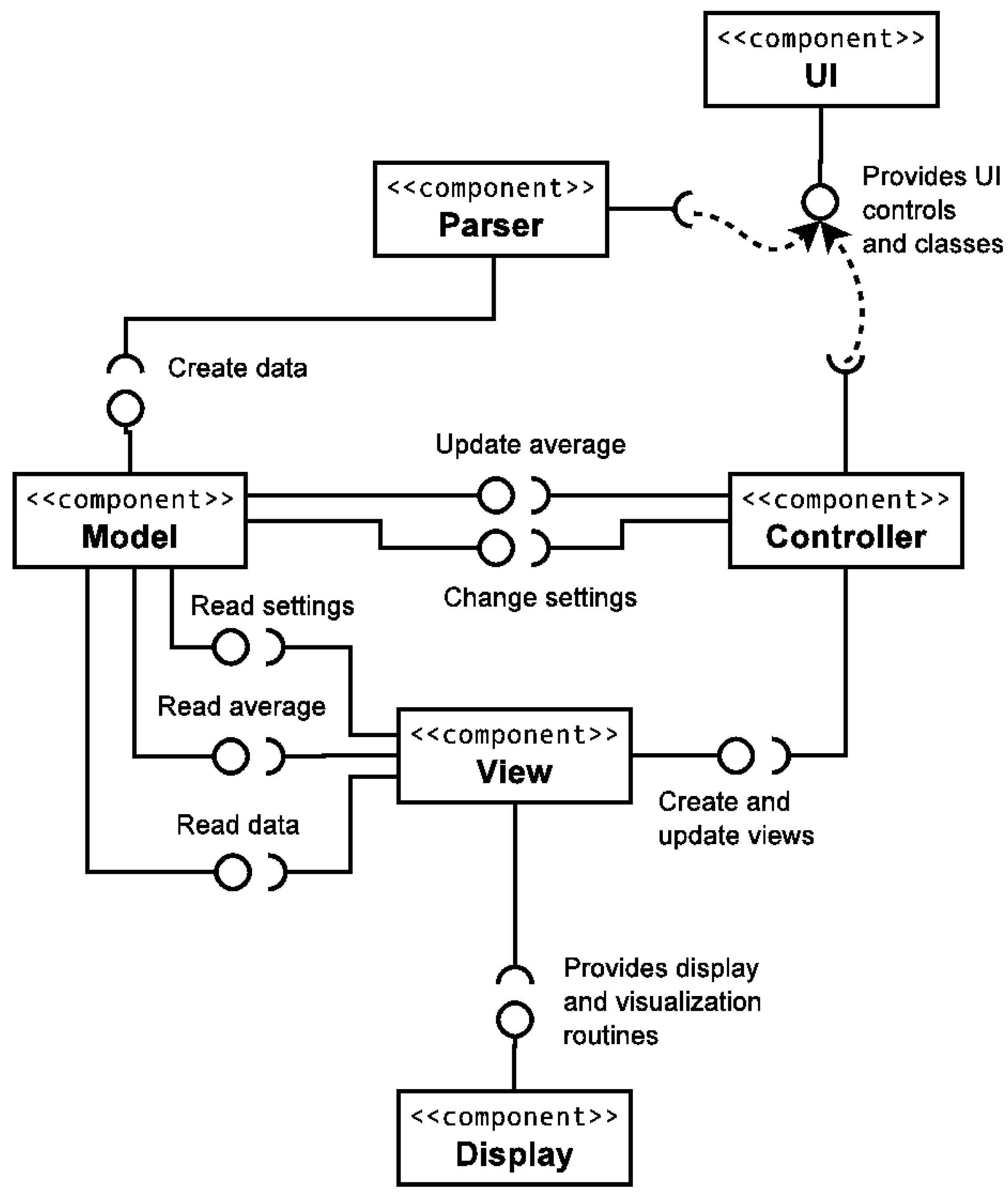
In this section, we present the structural relationships between FoamVis’ main components (
Figure 1). For this purpose, we use a UML (Unified Modeling Language), 2 component diagram [
10]. Briefly, a component represented in our diagram as a rectangle is a design unit that is typically implemented using a replaceable module. A component may provide one or more public interfaces, represented with a complete circle at their end (lollipop symbol). Provided interfaces represent services that the component provides to its clients. Similarly, a component may require services from other components. These services are formalized through the required interfaces, represented with a half circle at their end (socket symbol).
Figure 1.
FoamVis UML component diagram. The Parser parses simulation data and stores it in memory. FoamVis uses the model-view-controller design pattern to separate the data and program state (Model), the presentation (View) and the interaction with the user (Controller) into three different components. The UI provides user interface controls and classes, and the Display provides display and visualization algorithms.
FoamVis starts by executing the Parser component. This component, uses services from the UI component to allow the user to specify the simulations to be analysed and additional information about the simulations. This is done either through the command line or through the graphical user interface. Then, the Parser parses the specified simulation files, creates an in-memory representation of the simulation data and yields the execution to the Controller module.
The main logic of the program uses the model-view-controller design pattern [
11]. This pattern separates the data and program state (
Model), the presentation (
View) and the interaction with the user (
Controller) into three different components. This architecture has two main benefits. First, because views are separated from data, several views of the same data can be displayed at the same time. Second, because the
Model does not depend on the
View or
Controller components, changing the user interface or adding new views generally does not affect the
Model. This results in a more modular and maintainable code and in a quicker development cycle.
The Controller manages the interaction between a user, the Model (that stores the data and program state) and the views that show the foam simulation data.
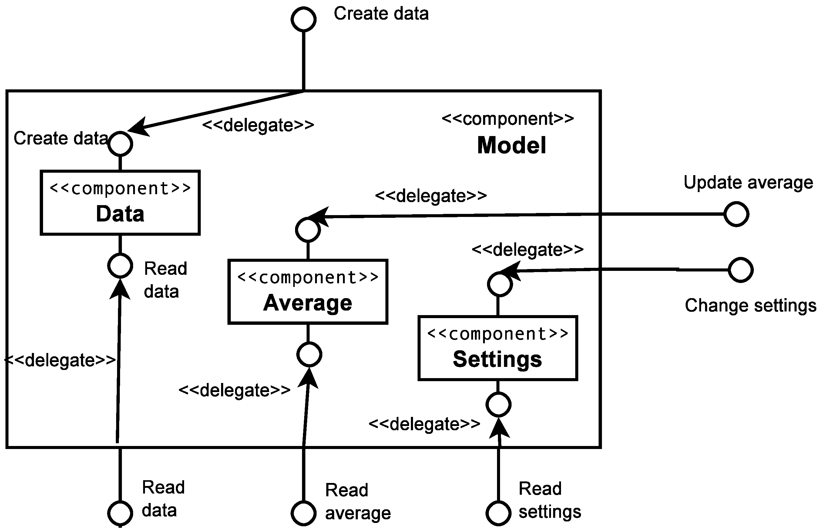
The
Model component (
Figure 2) is composed of three sub-components:
Data, which provides interfaces to create the in-memory representation of the foam simulation data and to read that data;
Settings, which stores the program state; and
Average, which stores and provides interfaces to compute and read the time averages of simulation attributes.
Figure 2.
The Model component. This component is responsible for storing the data and program state. It is composed of three subcomponents: Data, which stores the simulation data, Average, which stores the derived time average of simulation attributes, and Settings, which stores the program state.
Figure 2.
The Model component. This component is responsible for storing the data and program state. It is composed of three subcomponents: Data, which stores the simulation data, Average, which stores the derived time average of simulation attributes, and Settings, which stores the program state.
The View component provides visualizations for 2D and 3D foam simulation data, as well as histograms for scalar attributes.
Each of these logical components contains several implementation files, which, in turn, contain one or several related C++ classes. Logical components (modules), their implementation files and classes and groups of member functions (member groups) are also documented [
8] using Doxygen [
12]. We are going to refer to the Doxygen documentation as we describe the main features of the program and present implementation notes for those features. Here, we provide a brief summary of the main components of the program:
Parser,
Model,
View and
Controller. For brevity, we omit the
Display and
UI components. We include the name and a brief description for each file part of a component. We use a file name without an extension, to refer to both the interface (
.h) and the implementation (
.cpp) files with that name.
The
Parser parses Surface Evolver
.dmp files and calls the
Data component to build a memory representation of the simulation data. It contains the following files:
AttributeCreato: create attributes that can be attached to vertices, edges, faces and bodies.
AttributeInfo: information about attributes for vertices, edges, faces and bodies.
EvolverData.l: lexical analyser for parsing a .dmp file produced by Surface Evolver.
EvolverData.y: grammar for parsing a .dmp file produced by Surface Evolver.
ExpressionTree: nodes used in an expression tree built by the parser.
main.cpp: drives parsing of SE .dmp files and creates FoamVis main objects.
NameSemanticValue: tuple (name, type, value) used for a vertex, edge, face and body attribute.
ParsingData: stores data used during the parsing, such as identifiers, variables and functions.
ParsingDriver: drives parsing and scanning.
ParsingEnums: enumerations used for parsing.
The
Controller manages the interaction between a user, the
Model (that stores the data and program state) and the views that show the foam simulation data. This component contains one implementation file:
MainWindow: stores the OpenGL, Vtk and Histogram widgets, implements the Interface and manages the interaction between a user, the Model and the views.
The
Data component creates, processes and stores foam simulation data. It contains the following implementation files:
AdjacentBody: keeps track of all bodies of which a face is a part.
AdjacentOrientedFace: keeps track of all faces of which an edge is a part.
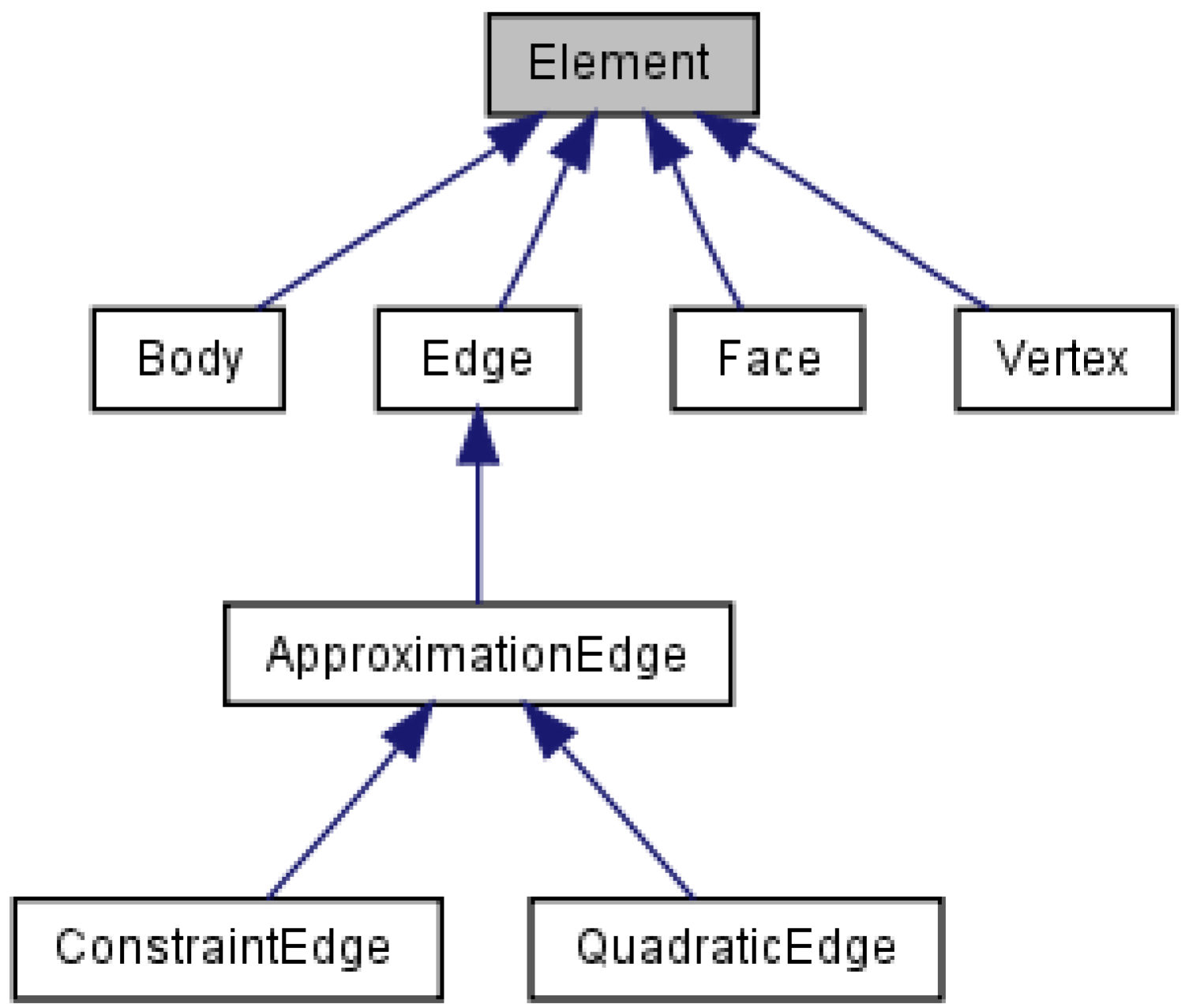
ApproximationEdge: curved edge approximated with a sequence of points (
Figure 3).
Attribute: attribute that can be attached to vertices, edges, faces and bodies.
Body: a bubble.
BodyAlongTime: a bubble path.
ConstraintEdge: edge on a constraint approximated with a sequence of points (
Figure 3).
DataProperties: basic properties of the simulation data, such as dimensions and if edges are quadratic or not.
Edge: part of a bubble face, stores a begin and an end vertex (
Figure 3).
Element: base class for Vertex, Edge, Face and Body; stores a vector of an attribute (
Figure 3)
Face: a bubble is represented as a list of faces; a face is an oriented list of edges.
Foam: stores information about a time step in a foam simulation.
ForceOneObject: forces and torque acting on one object.
ObjectPosition: stores an object interacting with foam position and rotation.
OOBox: an oblique bounding box used for storing a torus original domain.
OrientedEdge: an oriented edge; allows using an edge in direct or reversed order.
OrientedElement: base class for OrientedFace and OrientedEdge; allows using a Face or Edge in direct or reversed order.
OrientedFace: an oriented face; allows using a Face in direct or reversed order.
ProcessBodyTorus: processing done to “unwrap” bodies in the torus model.
QuadraticEdge: quadratic edge approximated with a sequence of points (
Figure 3).
Simulation: a time-dependent foam simulation.
T1: a topological change.
Vertex: element used to specify edges; an edge has at least two vertices, begin and end; a quadratic edge has a middle vertex, as well.
Figure 3.
Element class inheritance graph. This class stores a vector of attributes that can be attached to bodies (bubbles), faces, edges and vertices. This diagram also shows the three types of edges represented in FoamVis: regular (Edge) edges that have a begin and an end vertex, quadratic edges (QuadraticEdge) that have an additional middle vertex and constraint edges (ConstraintEdge) that are described using a begin vertex, an end vertex and a curve f (x, y, z) on which the edge lies.
The
Settings component stores and provides access to the program state. This component is composed of the the following files:
BodySelector: functors that specify selected bubbles.
Settings: settings that apply to all views.
ViewSettings: settings that apply to one view.
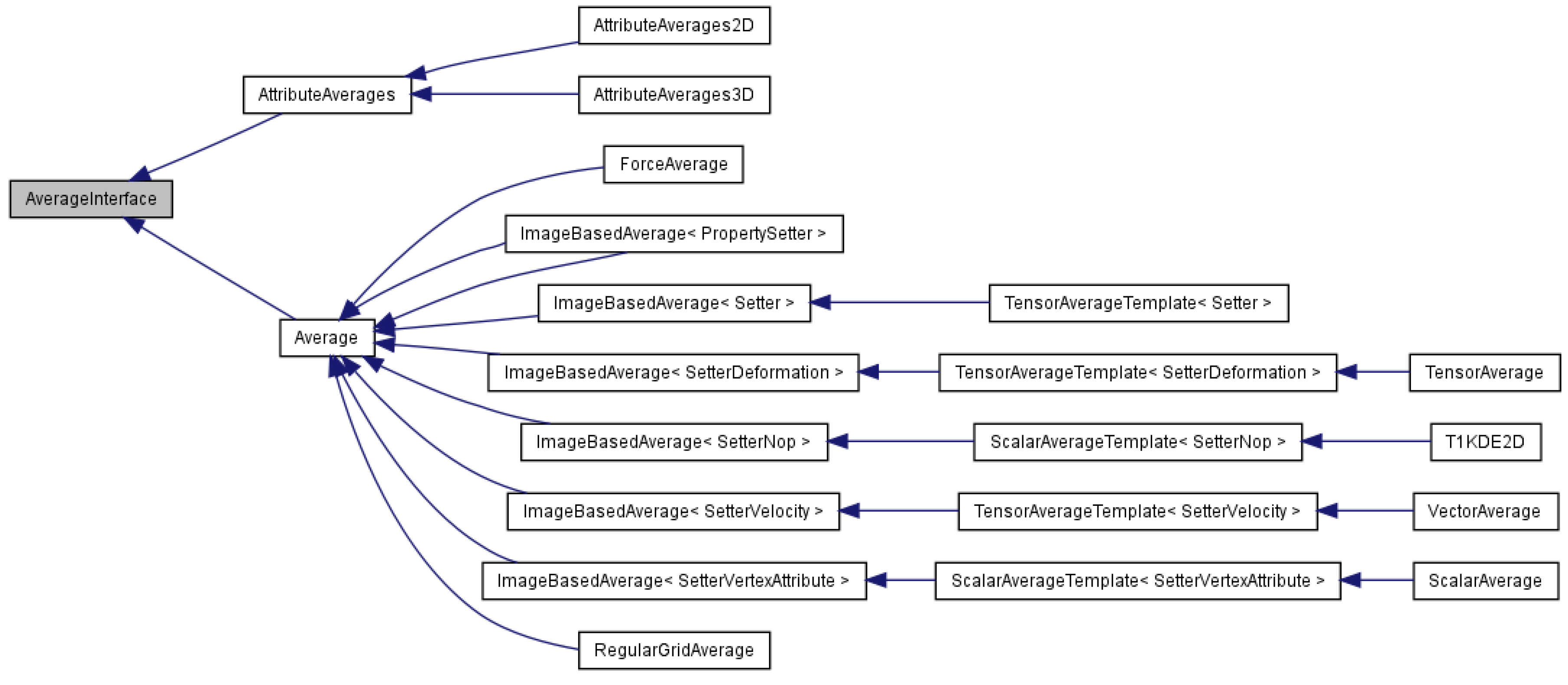
The
Average component computes the time average of simulation attributes. It contains:
AttributeAverages: computes the average for several attributes in a view; base class for AttributeAverages2D and AttributeAverages3D (
Figure 4).
AttributeAverages2D: computes the average for several attributes in a 2D view; casts the computed averages to the proper 2D types (
Figure 4).
AttributeAverages3D: computes the average for several attributes in a 3D view; casts the computed averages to the proper 3D types (
Figure 4).
Average: computes a time average of a foam attribute; base class for 2D and 3D time average computation classes (
Figure 4).
AverageInterface: interface for computing a time average of a simulation attribute (
Figure 4).
AverageShaders: shaders used for computing a pixel-based time average of attributes.
ForceAverage: time average for forces acting on objects interacting with foam (
Figure 4).
ImageBasedAverage: calculates a pixel-based time average of 2D foam using shaders (
Figure 4).
PropertySetter: sends an attribute value to the graphics card (
Figure 4).
RegularGridAverage: time average for a 3D regular grid (
Figure 4).
ScalarAverage: computes 2D scalar average (
Figure 4).
T1KDE2D: calculates T1 KDE for a 2D simulation (
Figure 4).
TensorAverage: computes a pixel-based time average of vector and tensor attributes (
Figure 4).
VectorAverage: computes a pixel-based time average of vector attributes (
Figure 4).
VectorOperation: math operations for vtkImageData, used for 3D average computation.
Figure 4.
AverageInterface inheritance graph. This class provides the interface for updating an average of attributes. AttributeAverages stores an average of many simulation attributes Average provides common computation for averages of forces (ForceAverage), 2D simulation attributes (ImageBasedAverage) and 3D simulation attributes (RegularGridAverage). Two-dimensional averages include scalars (ScalarAverage), vectors (VectorAverage), tensors (TensorAverage) and kernel density estimates (T1KDE2D).
The
Model component consists of the
Data,
Settings and
Average components. It also includes two additional files:
Base: simulation data, derived data and program status.
DerivedData: data derived from simulation data, such as caches and averages.
The
View component contains the views for displaying data. It contains the following implementation files:
AttributeHistogram: a GUI histogram of a scalar attribute useful for one time step and all time steps.
FoamvisInteractorStyle: interactor that enables FoamVis style interaction in a VTK (Visualization Tool Kit) [
13] view.
Histogram: a histogram GUI that allows the selection of bins.
HistogramItem: implementation of a GUI histogram, modified from Qwt (Qt Widget Graphing Library) [
14].
WidgetBase: base class for all views: WidgetGl, WidgetVtk, WidgetHistogram.
WidgetGl: view that displays 2D (and some 3D) foam visualizations using OpenGL.
WidgetHistogram: view for displaying histograms of scalar values.
WidgetSave: widget that knows how to save its display as a JPG file.
WidgetVtk: view that displays 3D foam visualizations using VTK.
3.2. Parsing and Data Processing
Foam simulation data consist of a list of SE output files, one per time step. A file stores the entire configuration of the simulated foam at a particular time step. For maximum generality and flexibility, we parse SE files directly instead of using derived files created by foam scientists. This allows our application to work with any simulation created using SE, and at the same time, it gives us access to the entire duration and state of the simulation. Parsing is done using
flex [
15] and
bison [
16] tools using the
EvolverData.l lexical analyser and
EvolverData.y grammar. Parsing is run by
Simulation::ParseDMPs, which parses the simulation files, stores the simulation data in memory and performs the additional processing required.
Our tool can read the following optional data that is saved by the simulation code: a list of T1s and the network and pressure forces that act on a body (
Section 3.4).
After parsing foam simulation data and creating the corresponding data structures, we perform additional data processing (
Foam::Preprocess and
Simulation::Preprocess). First, we compact each list of geometric elements, as there can be numbering gaps in the list specified in an SE file (
Foam::compact). Then, if the foam described in the SE file contains periodic boundary conditions (PBC) [
17,
18], we unwrap the geometric elements, so that we can display the foam (
Foam::unwrap). Additional processing include calculating each bubble’s centre of mass (
Foam::calculateBodyCenters), the bounding box and the bounding box of the foam at each time step (
Foam::CalculateBoundingBox and overall (
Simulation::CalculateBoundingBox and calculating statistical quantities, such as histogram, minima and maxima, for values of attributes (
Simulation::calculateStatistics). For 3D foam simulations, unstructured simulation data are converted to a regular grid, and it is cached in files on disk (
Section 3.6).
The design of the data structures for storing bubbles and their topology is object oriented. We have an object that stores an instance of each bubble. The Bubble contains a list of edges. These are the shared edges between neighbouring bubbles. The Bubble object also stores a pointer to its neighbouring bubbles. Technically speaking, this information could be considered redundant, since bubbles share edges; however, it does accelerate computation. Another option is to have each edge contain a list of pointers to its bubble objects. This is an important consideration for neighbour searching. During the foam evolution, the foam topology must be updated for every T1 event.
3.3. Interface
Each dataset consists of a list of data files stored in a folder. The only information about the simulation available without parsing the simulation files is the name of the folder. While this often encodes important parameters of the simulation, their meaning may be cryptic and only known to the scientist that created the simulation. Additionally, there is an increasing number of parameters providing additional information about the simulation, which is not encoded in the simulation files. To address these issues, we create a simulation database and a browsing interface. The simulation database records for each simulation three pieces of information: a simulation name (usually, this is the name of the folder that stores the simulation files); a list of labels (each label is used to group simulations based on specific criteria); and simulation-specific visualization parameters. The database is stored as a .ini file and is created by the user from a template. The UI, Options file contains classes that read options either from the command line or from an .ini file.
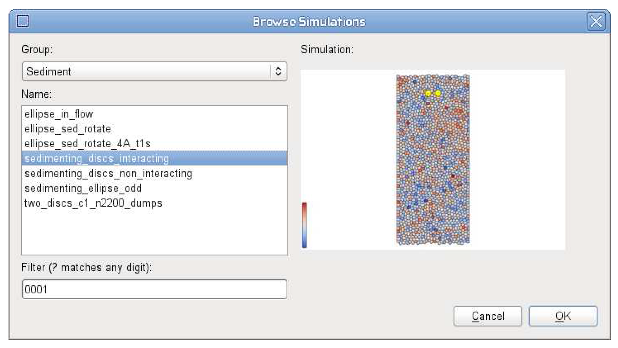
The browsing feature (
Figure 5) presents all grouping labels from the simulation database in a list. When a user selects a label, a list with all simulations tagged by that label is presented. When a user selects a simulation name, a picture of the first time step in the simulation is displayed. The image is saved beforehand, so no parsing of simulation files is required. This allows a user to explore existing simulations based on similarity criteria encoded in labels and to visually select simulations of interest for individual analysis or comparison.
Figure 5.
The BrowseSimulations dialogue, which allows the user to view related simulations and select simulations of interest for individual analysis or comparison.
Figure 5.
The BrowseSimulations dialogue, which allows the user to view related simulations and select simulations of interest for individual analysis or comparison.
The browsing dialogue is implemented by the UI, BrowseSimulations class.
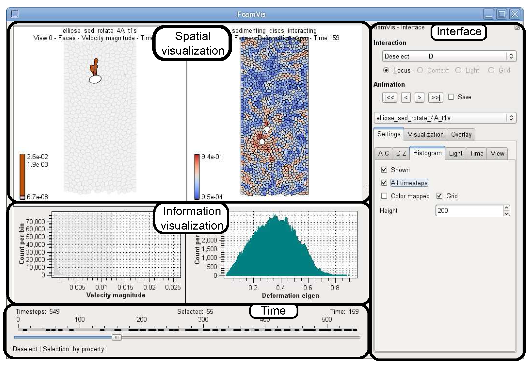
FoamVis’ main window (
Figure 6) contains three panels that are used for both visualization and user interaction (spatial and information visualization and time) and one panel (Interface) that allows the user to specify desired visualizations and visualization parameters. The spatial visualization panel shows multiple views, with each view showing a different visualization, a visualization of a different simulation attribute or a visualization of a different simulation. The information visualization panel shows histograms for simulation scalars shown in the spatial visualization panel. The time panel shows the current time step and marks the time steps resulting from selections on scalar values.
The main window of the application is implemented in
Controller,
MainWindow. This class implements the Interface panel and handles user notifications resulting from user interactions with the panel or with simulation data. The spatial visualization panel is implemented by the
View component. In this component, the
WidgetGl class displays 2D visualizations and 3D attribute and bubble path visualizations; the
WidgetVtk class displays 3D attribute time average and T1 KDE visualizations. The decision to use VTK [
13] rather than plain OpenGL [
19] for some of the 3D visualizations was based on the desire to speed-up the development of the application. We believe this was a sound decision, which, besides speeding-up development, opened up a wide range of visualization algorithms for adoption into FoamVis.
Figure 6.
FoamVis’ MainWindow showing the spatial visualization, information visualization, time and interface panels. The spatial visualization panel shows two views: bubble velocity magnitude for a falling ellipse simulation and bubble deformation for a falling discs simulation. A selection of velocity magnitude values is performed on the histogram showing this scalar, and it is reflected in the spatial visualization and time panels. We can observe in the time panel that only 55 time steps out of 549 contain high velocity bubbles, and in the spatial visualization panel, we see those bubbles colour mapped; the rest of the bubbles are rendered in grey as context information.
3.4. Simulation Attributes
Scalar bubble attributes include velocity along principal axes, velocity magnitude, edges per face, deformation, pressure, volume and growth rate. Scalar bubble attributes are visualized using colour mapping. The user can change the colour palette and change the range of scalar values mapped to colour through clamping (
Section 3.10).
Figure 7a,
Figure 8 and
Figure 6 show examples of scalar attributes visualized through colour mapping. While domain experts are mostly interested in bubble attributes, in SE, attributes can be attached to a body (bubble), face, edge or vertex. Information about predefined attributes that can be attached to one of these elements is stored in the
Parser,
AttributesInfoElements class. New attributes can be defined in a
.dmp file. The
Parser calls
Data,
Foam::AddAttributeInfo to register a new attribute. The
Parser,
EvolverData.y parses a list of attributes on the following grammar rules:
xxx_attribute_list, where
xxx is the vertex, edge, face or body. It creates a list of
NameSemanticValue objects, and it passes them to the
Foam object for storage.
Bubble velocity, defined as the motion of the centre of mass, provides information about foam flow. We visualize bubble velocities using glyphs (2D and 3D) (
Figure 7a) and streamlines (2D only) (
Figure 9). We compute the velocity attribute in a processing step after parsing (
Simulation::Preprocess) in
Simulation::calculateVelocity. Velocity glyphs are visualized using the
Display module,
DisplayBodyFunctors file and
DisplayBodyVelocity class.
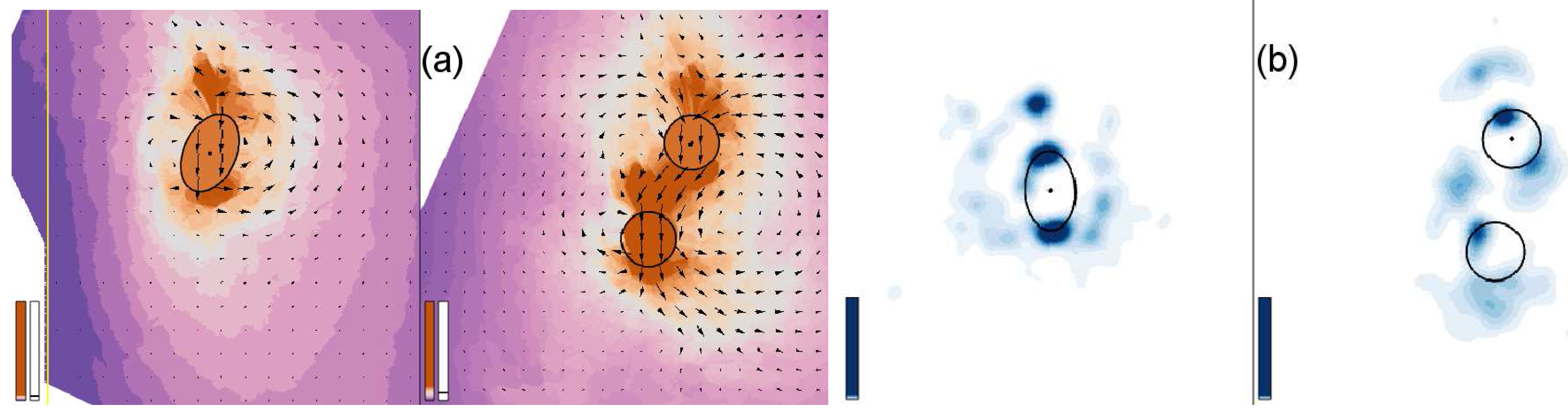
Figure 7.
Are the falling discs behaving like the falling ellipse? (
a) The foam between the discs moves at high velocity with the discs. Velocity is displayed using glyphs, and velocity magnitude is also colour-mapped. (
b) Few topological changes occur between the discs, so the foam behaves like an elastic solid there. Topological changes over time visualized using the kernel density estimate (KDE) [
7].
Bubble deformation magnitude and direction are important bubble attributes, because they facilitate the validation of simulations and provide information about the force acting on a dynamic object in foam. While visual inspection of individual bubbles provides information about foam deformation, this information is not quantified and, more importantly, cannot be averaged to obtain the general foam behaviour. To address these issues, we define a bubble deformation measure [
7] expressed as a tensor. The deformation tensor is visualized using glyphs, as shown in
Figure 8. We compute a deformation scalar and tensor measures in a processing step after parsing:
Foam::CalculateDeformationSimple and
Foam::CalculateDeformationTensor. Two-dimensional deformation glyphs are visualized using the
Display module,
DisplayBodyFunctors file and
DisplayBodyDeformation class.
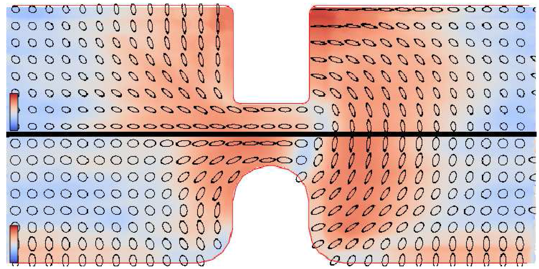
Figure 8.
Rounding the corners of the constriction results in reduced elastic deformation of the foam (top
versus bottom). In both simulations, there is an area where bubbles are not deformed just downstream from the constriction. We show the square (top) and rounded (bottom) constriction simulations. Deformation magnitude and direction is displayed with ellipses; deformation magnitude is also colour-mapped. An average over the entire duration of the simulations is displayed [
7].
When foam is subjected to stress, bubbles deform (elastic deformation) and move past each other (plastic deformation). Domain experts are interested in the distribution of the plasticity, which is indicated by the location of topological changes. A topological change is a neighbour swap between four neighbouring bubbles. In a stable configuration, bubble edges meet three-way at 120° angles. As foam is sheared, bubbles move into an unstable configuration, in which edges meet four-way, then quickly shift into a stable configuration. Topological changes for the current time step or for all time steps are visualized with glyphs (or spheres) of configurable colour and size showing the location of the topological change (
Figure 9). Topological changes are parsed either from a separate file or from variables inside the
.dmp file by the overloaded function
Simulation::ParseT1s. They are stored in the
Simulation object.
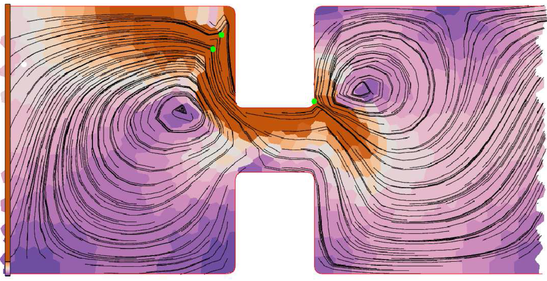
Figure 9.
Topological changes are associated with strong circulation; topological changes shown with green dots; velocity field shown with streamlines, t = 412. Velocity is shown with streamlines, and velocity magnitude is colour-mapped.
Figure 9.
Topological changes are associated with strong circulation; topological changes shown with green dots; velocity field shown with streamlines, t = 412. Velocity is shown with streamlines, and velocity magnitude is colour-mapped.
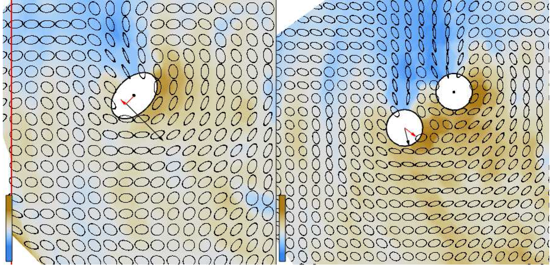
The forces and the torque acting on objects are computed by the simulation code and stored in the simulation data. Each force acting on an object is represented with an arrow that starts in the centre of the object and with a length proportional to the magnitude of the force.
For the falling discs simulation, the interplay of the network and pressure forces rotate one disc around the other. We provide a user option that displays the difference between the forces acting on the leading disc and forces acting on the trailing disc. This difference allows us to better analyse the causes of the rotation, as there is a direct correspondence between the forces displayed on the screen and the movement of the disc (
Figure 10 right).
Figure 10.
Falling-ellipse
versus falling-discs. The linked time with event synchronization feature [
7] is used to synchronize the rotation of the ellipse and the two discs, such that they reach an orientation of 45° in the same time. Attributes (pressure, deformation and forces) are averaged over 52 time steps for the ellipse simulation (resulting in an average of over 15 time steps for the two disc simulation). Pressure is colour-mapped; deformation is shown using ellipses. The force difference between the leading disc and the trailing disc and the torque on the ellipse is indicated. The network force and torque are indicated with a black arrow, and the pressure force and torque are indicated with a red arrow.
The torque
τ rotating an object around its centre is displayed as a force
F acting off-centre on the object
τ =
r × F, where
r is the displacement vector from the centre of the object to the point at which the force is applied. The distance
|r| is a user-defined parameter; FoamVis calculates the appropriate value of
F to keep the torque constant (
Figure 10 left).
The forces and torques acting on objects are read from the simulation files, from variable names passed as parameters either from the command line or from the .ini file. Variable names that store forces and torques are passed as parameters in the Data, ForceNamesOneObject class, while the forces and torques are stored in Data, ForceOneObject in the Foam object. Forces are displayed using ForceAverage::DisplayOneTimeStep for OpenGL views or using PipelineAverage3D::createObjectActor for VTK views. This function would better fit in the Display module, as this would separate the data from its display. We plan to address this issue in future work.
3.6. Time Average of a Simulation Attribute
Bubble-scale simulations can be too detailed for observing general foam behaviour, and topological changes generate large fluctuations in attribute values that hide the overall trends. A good way to smooth out these variations is to calculate the average of the simulation attributes over all time steps or over a time window before the current time step. This visualization reveals global trends in the data, because large fluctuations caused by topological changes are eradicated. This results in only small variations between averaged successive time steps. The time window is a parameter set by the user. We compute the average for the entire simulation (
Figure 8) if there are no dynamic objects interacting with the foam. In this case, at a high level of detail, there is no difference between different time steps in the simulations. For simulations that include dynamic objects interacting with the foam (
Figure 7 and
Figure 10), a smaller time window is appropriate, as objects may traverse transient states that have to be analysed independently.
Time averages of several 2D foam simulation attributes are stored in
AttributeAverages2D and are referenced from
WidgetGl. A pixel-based time average of one simulation attribute is computed by
ScalarAverage,
VectorAverage and
TensorAverage for scalars, vectors and tensors. Most of this computation is done in the base class
ImageBaseAverage (
Figure 4). Displaying an average of attributes is done by the graphics card fragment shader using
AverageInterface::AverageRotateAndDisplay overwritten for each attribute type. For 3D simulations, unstructured grid data are converted to regular grid data and are cached in files inside the
.foamvis folder using
Foam::SaveRegularGrid. This is done in the processing step after parsing
Simulation::Preprocess. Time averages of several 3D foam simulation attributes are stored in
AttributeAverages3D and are referenced from
WidgetVtk. A time average for one attribute, for all types of attributes is computed by
RegularGridAverage and displayed using a VTK pipeline created by
PipelineAverage3D::createScalarAverageActor and
PipelineAverage3D::createVelocityGlyphActor for scalars and respective vectors.
3.7. Topological Change Kernel Density Estimate
Topological changes, in which bubbles change neighbours, indicate plasticity in a foam. Domain experts expect that their distribution will be an important tool for validating simulations. Simply rendering the position of each topological change suffers from over-plotting, so it may paint a misleading picture of the real distribution. We compute (see Lipsa
et al. [
7] for details) a KDE for topological changes (
Figure 7 and
Figure 12). While traditional histograms show similar information and are straightforward to implement, they have drawbacks, which may prove important, depending on the context. The drawbacks of histograms include the discretization of data into bins, which may introduce aliasing effects, and the fact that the appearance of the histogram may depend on the choice of origin for the histogram bins [
20,
21]. Kernel-based methods for computing the probability density estimation eliminate these drawbacks.
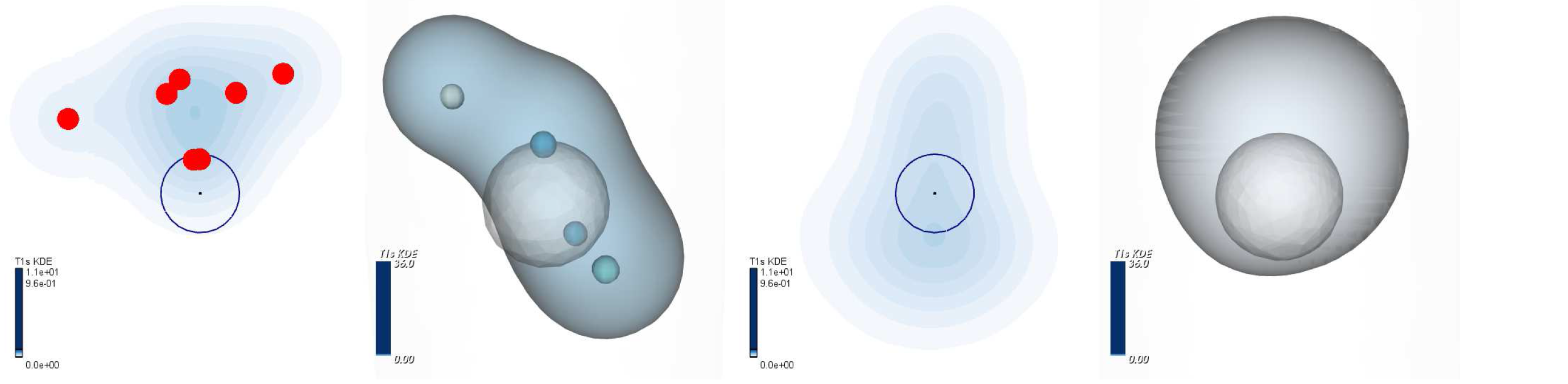
Figure 12.
KDE around the falling disc versus falling sphere simulations. (Left) The KDE for one time step: t = 18 left view and t = 21 right view. The isosurface density is 0.5 for the right view. The maximum values in the colour bar represent the maximum number of topological changes in a time step. KDE for all time steps (Right) shows that, for 3D, topological changes on top of the sphere dominate the final result. This is caused by topological changes in the same area being triggered repeatedly in the simulation code feature discovered using our visualization. The isosurface density is 0.12 for the right view
T1s KDE is computed using the average framework (
Figure 4) (
T1KDE2D or
RegularGridAverage classes for 2D or 3D foam simulation). For 2D simulations, for each topological change in a time step, a Gaussian is added to the average using
T1KDE2D::writeStepValues. For 3D simulations, a Gaussian determined by a topological change in a time step is returned by
Simulation::GetT1KDE. This Gaussian is added to the current average in
RegularGridAverage::OpStep.
3.9. Multiple Linked Views
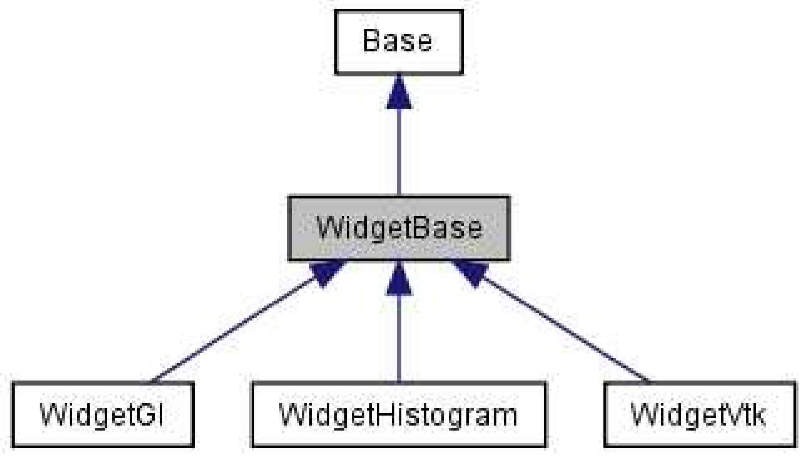
Foam scientists wish to understand what triggers certain behaviour in foam simulations. Foam behaviour is determined by many simulation attributes, so the ability to see different attributes at the same time and to understand how different attributes relate to one another is very important. At the same time, to understand the influence that simulation parameters have on foam behaviour, foam scientists would like to analyse and compare related simulations. Both of these requirements are addressed using multiple linked views. We provide up to four different views. For maximum flexibility, each view can depict a different simulation attribute, a different visualization or even a different simulation. Each view uses its own colour-bar and can show the navigation context. Each of the three widgets used to show data (
WidgetGl,
WidgetVtk and
WidgetHistogram) can display up to four views. These three classes are derived from
WidgetBase, which provides view-related functionality; WidgetBase is derived from
Base, which provides access to the data and program status (
Figure 13).
Figure 13.
WidgetBase inheritance graph. This class provides functionality common to all views. It inherits from Base, which stores the simulation data and program status. WidgetGl displays views rendered with OpenGl. WidgetVtk displays views rendered with VTK, and WidgetHistogram displays histograms.
To set up optimal views to analyse data, users can copy viewing transformations and colour mapping between views depicting the same attribute (MainWindow::CopyColorMapXXX, where XXX is scalar or velocity).
The two halves option facilitates the visual comparison of two related foam simulations (
Figure 8). It visualizes related simulations that are assumed to be symmetric with respect to one of the main axes. While the same information can be gathered by examining the two simulations in different views, the two halves view may facilitate analysis, as images to be compared are closer together, and it is useful for presentation, as it saves space. This type of visualization was previously performed manually by domain experts. This option is only available for 2D simulations in
WidgetGl. It is set using
Settings::SetTwoHalvesView.
We provide three connection operations [
22] between views: one linked-selection connection and two linked-time connections. The linked-selection connection works by showing data selected in one view in other views. This is used to see, for instance, the elongation of high pressure bubbles or both pressure and elongation for bubbles involved in a topological change. This connection works by copying the selection in one view in any other view using
ViewSettings::CopySelection.
The first linked-time connection works by having each view linked to the same time step, as foam scientists want to analyse several attributes at the same time to understand the foam behaviour influenced by those attributes. The linked-time connection is set to independent time or linked time using
Settings::SetTimeLinkage. The second linked-time connection, linked-time with event synchronization, is described next. In simulations that involve dynamic objects interacting with foam, we may want a similar event in both simulations to be visualized at the same time, so that behaviour up to that event can be compared and analysed together. When comparing the falling discs with the falling ellipse simulations, the ellipse and the discs start in similar configurations. The main axis of the ellipse and the line connecting the centre of the two discs are horizontal. We want the ellipse and the discs to reach intermediate configurations and the stable configuration at the same time. These configurations are defined in terms of the angle that the major axis of the ellipse and the line connecting the centres of the two discs make with gravity. For instance, an angle for the intermediate configuration could be 45°, while the angle for the stable configuration is 0°. A new event for the current view and current time is added using
Settings::AddLinkedTimeEvent. All views that use linked-time with event synchronization have to have the same number of events. This technique splits simulation times into intervals: an interval before each event and an interval after the last event. For each interval before an event, one simulation will run at its normal speed (the simulation with the longest interval as returned by
Settings::GetLinkedTimeMaxInterval), and all other simulations will be “slowed down” using
Settings::GetLinkedTimeStretch. Simulations will run at normal speed for the time interval after the last event. Using this approach, related events occur at the same linked time in all simulations, facilitating their comparison, as well as the comparison of their temporal context.
Figure 7 and
Figure 10 use linked-time with the event synchronization feature. The complete interface for using the linked-time with event synchronization is in class
Settings, member group
Time and
LinkedTime.
3.10. Interaction
Interaction with the data is an essential feature of our application.
Navigation is used to select a subset of the data to be viewed, the direction of view and the level of detail [
22]. We provide the following navigation operations: rotation around a bounding box centre for specifying the direction of view and translation and scaling for specifying the subset of data and the level of detail. Navigation operations are implemented in the
WidgetGl views in
mousePressEvent and
mouseMoveEvent. These operations are provided by the VTK library in the
WidgetVtk views. A navigation context (
Figure 11 left) ensures that the user always knows its location and orientation during the exploration of the data. Focus and context-related settings are in the
ViewSettings,
Context view.
We can select and/or filter bubbles and centre paths based on three distinct criteria: based on bubble IDs (
WidgetGl::SelectBodiesByIds), to enable data to be related to the simulation files and for debugging purposes; based on the location of bubbles (
WidgetGl::mousePressEvent and
WidgetGl::mouseMoveEvent), to analyse interesting features at certain locations in the data; and based on an interval of attribute values specified using the histogram tool (
Figure 6) (the histogram sends the
WidgetHistogram::selectionChanged signal, which is handled in
MainWindow::SelectionChangedFromHistogram). A composite selection can be specified using both location and attribute values.
Selected bubbles or centre paths constitute the focus of our visualization, and the rest of the bubbles or centre paths provide the context [
23]. The context of the visualization is displayed using user-specified semi-transparency, or it can be hidden altogether.
Encoding operations are variations of graphical entities used in a visualization that emphasize features of interest [
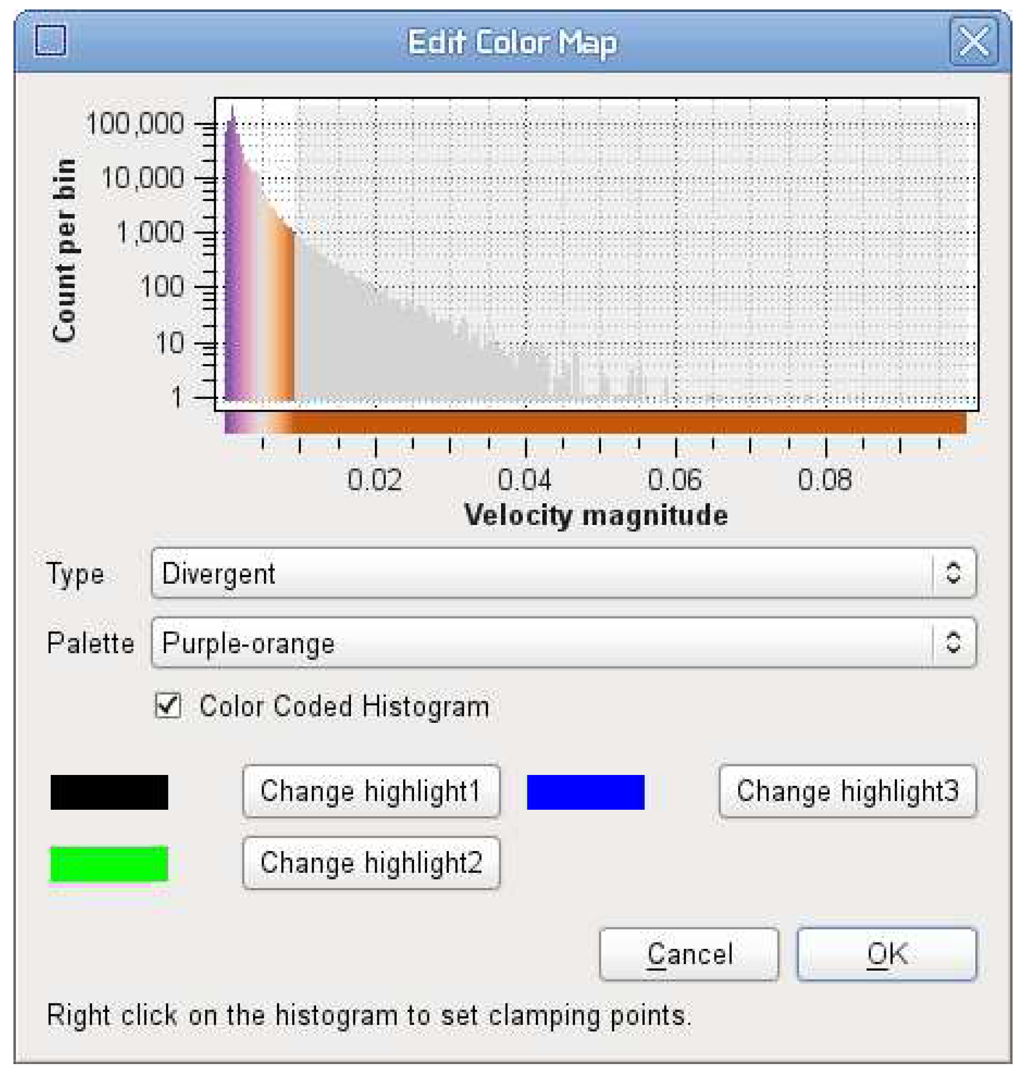
22]. We provide encoding operations to change the colour map used, to specify the range of values used in the colour map and to adjust the opacity of the visualization context. Selection of the interval used in colour-mapping is guided by the histogram tool (
Figure 14) (the implementation is in
EditColorMap). This provides essential information for selecting an interval that reveals the features of interest.
Figure 14.
Colour-map clamping guided by the histogram tool (EditColorMap class). This is a histogram of the constriction simulation, which uses a logarithmic height scale. The histogram is clamped at high values. The dialogue also allows the user to choose a different colour palette and to change the highlight colours used for vector and tensor glyphs and the forces acting on objects.


