Article

Potential of Forest Parameter Estimation Using Metrics from Photon Counting LiDAR Data in Howland Research Forest

1
Institute of Forest Resource Information Techniques, Chinese Academy of Forestry, Beijing 100091, China
2
Global Environmental Modelling and Earth Observation (GEMEO), Department of Geography, Swansea University, Swansea SA2 8PP, UK
3
Department of Geographical Sciences, University of Maryland, College Park, MD 20742, USA
4
Forest Research, Northern Research Station, Roslin, Midlothian EH25 9SY, Scotland, UK
5
School of Information Science and Technology, Beijing Forestry University, Beijing 100083, China
*
Author to whom correspondence should be addressed.
Remote Sens. 2019, 11(7), 856; https://doi.org/10.3390/rs11070856
Submission received: 18 February 2019 / Revised: 6 April 2019 / Accepted: 7 April 2019 / Published: 9 April 2019
(This article belongs to the Section Forest Remote Sensing)

Abstract

:
ICESat-2 is the new generation of NASA’s ICESat (Ice, Cloud and land Elevation Satellite) mission launched in September 2018. We investigate the potential of forest parameter estimation using metrics from photon counting LiDAR data, using an integrated dataset including photon counting LiDAR data from SIMPL (the Slope Imaging Multi-polarization Photon-counting LiDAR), airborne small footprint LiDAR data from G-LiHT and a stem map in Howland Research Forest, USA. First, we propose a noise filtering method based on a local outlier factor (LOF) with elliptical search area to separate the ground and canopy surfaces from noise photons. Next, a co-registration technique based on moving profiling is applied between SIMPL and G-LiHT data to correct geolocation error. Then, we calculate height metrics from both SIMPL and G-LiHT. Finally, we investigate the relationship between the two sets of metrics, using a stem map from field measurement to validate the results. Results of the ground and canopy surface extraction show that our methods can detect the potential signal photons effectively from a quite high noise rate environment in relatively rough terrain. In addition, results from co-registration between SIMPL and G-LiHT data indicate that the moving profiling technique to correct the geolocation error between these two datasets achieves favorable results from both visual and statistical indicators validated by the stem map. Tree height retrieval using SIMPL showed error of less than 3 m. We find good consistency between the metrics derived from the photon counting LiDAR from SIMPL and airborne small footprint LiDAR from G-LiHT, especially for those metrics related to the mean tree height and forest fraction cover, with mean R 2 value of 0.54 and 0.6 respectively. The quantitative analyses and validation with field measurements prove that these metrics can describe the relevant forest parameters and contribute to possible operational products from ICESat-2.

Graphical Abstract

1. Introduction

The reliable and accurate estimation of important forest parameters such as forest height and canopy cover is crucial for understanding the global carbon stock and cycle [1,2,3,4,5]. LiDAR (Light Detection And Ranging) has demonstrated the capability to detect the vertical structure of forests with high accuracy [6,7,8,9], and a spaceborne LiDAR system would significantly contribute to the continued long term vegetation monitoring over large spatial context. The relevant studies using the data from the Geoscience Laser Altimeter System (GLAS) system onboard the NASA’s ICESat (Ice, Cloud and Land Elevation Satellite) mission showed very promising results in vegetation studies [10,11,12,13]. Several global vegetation products focused on the key forest parameters were produced by combining with GLAS data and other source data [14,15], and the data remain actively used even after the failure of the laser sensors.
ICESat-2, the new generation of ICESat missions, was launched in September 2018 [16]. In contrast with the previous waveform LiDAR system [17], ICESat-2 will use a new photon counting approach adopted for the first time on a spaceborne platform. This newly designed system is named ATLAS (Advanced Topographic Laser Altimeter System), which is a micro-pulse, multi-beam photon counting LiDAR working at 532 nm [18]. To investigate the expected performance and develop relevant algorithms for this new sensor, several spaceflight prototype instruments including SIMPL (The Slope Imaging Multi-polarization Photon-counting LiDAR) [19] and MABEL (the Multiple Altimeter Beam Experimental LiDAR) [20,21] were designed and tested in airborne flight campaigns over the past few years [22], and a large collection of relevant data products were archived.
There have already been studies to explore the current released ATLAS-like data from the airborne prototype. These studies show that one of the challenges for application to vegetation study is the significant quantity of noise photons, with photon return time giving the appearance of originating in the atmosphere and even below the ground [23,24]. Several attempts have been made to separate the signal photons from the noise photons by methods such as spatial statistical based detection algorithms, Density-Based Spatial Clustering of Applications with Noise (DBSCAN), ellipsoidal histogramming method, and a framework to retrieve ground and canopy height [25,26,27,28,29]. In addition, some studies focused on the application rather than the data pre-processing showed some promising results, especially for vegetation studies [30,31,32,33]. However, studies focusing on the potential estimation of forest parameters by using the ATLAS-like data are still very limited. There are some findings including investigating the dryland ecosystem vegetation cover and biomass by using a combination of Landsat 8 and ATLAS-like data [34], the similarity comparison with airborne LiDAR system of the ICESat-2 laser altimetry for savanna ecosystem [28,35], and an automated approach for better estimating vegetation canopy height [36]. The study to explored potential for biomass retrieval over boreal ecosystems, using the radiative transfer model FLIGHT to simulate ICESat-2 [37].
These studies have shown some promising results of the potential of photon counting LiDAR, but a comprehensive analysis in terms of different forest parameters focusing on SIMPL data is very limited. In this context, the Eco3D SIMPL flight campaign produced some valuable datasets but these are not yet fully analyzed. The flight path coincides with the data coverage of Goddard’s LiDAR, Hyperspectral and Thermal Imager (G-LiHT) and Howland stem map, which has tremendous ecological value having escaped the mechanized logging that characterizes the northern forests of Maine. In addition, although ICESat-2 has been successfully launched last year, the data products are still not publicly available to access. Also, it would require a period of time to cover some typical forest types such as the northern forests of Maine. Therefore, it still remains a good aim to concentrate on the existing simulation data, of which the 532 nm data from SIMPL is a good testing data because it has the same working wavelength as ATLAS. In these circumstances, relevant researches to explore the potential of forest parameter estimation using SIMPL data would be of use for the future applications of ICESat-2 vegetation studies.
This study investigates the potential of forest parameter estimation using metrics from photon counting LiDAR data, by using a combination of SIMPL, G-LiHT, and field measurement data collected in Howland Research Forest. To achieve this goal, we develop pre-processing methods to extract the canopy photon surface and co-registration with G-LiHT data, we further propose a set of photon metrics and examine the consistency and accuracy with airborne small footprint LiDAR data. Finally we quantitatively analyze the results and validate with field measurements.

2. Study Site and Data
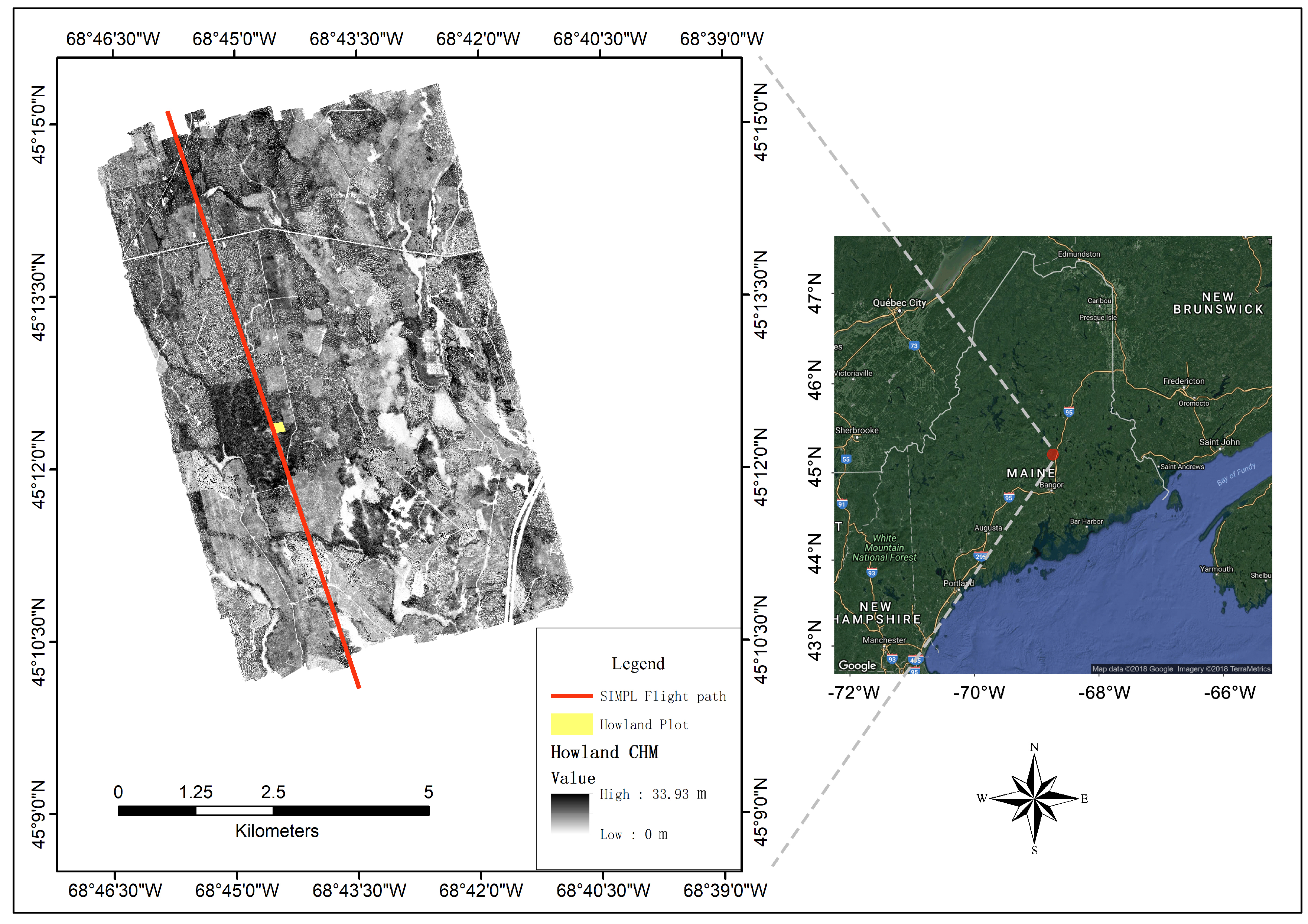
2.1. Study Site

The Howland Research Forest is a 558 acre tract of mature, lowland evergreen forest located in central Maine, west of the town of Howland. Red spruce, Eastern hemlock and white cedar trees dominate the forest canopy. Stands contain large amounts of woody biomass (up to 350 Mg/ha), standing and downed dead trees, and pit-and-mound topography created by tree tip-over. The tract of land was designated as a research forest in 1986, and has tremendous ecological value having escaped the mechanized logging that characterizes the northern forests of Maine. A 29 m walkup flux measurement tower has been in operation since the 1980s. Near the flux tower, every tree in a 200 m by 150 m area was measured for its location, DBH (Diameter at Breast Height), and species in 1989, 2003 and measured again in 2010.
Figure 1 shows the location and data obtained for this study, including: (1) the photon counting LiDAR data from the Eco3D SIMPL flight path on 1 September 2011; (2) the airborne small footprint LiDAR data from the G-LiHT in 2012; (3) the stem map based on the measurements in 2010 used to conduct the validation.

2.2. Photon Counting LiDAR Data from SIMPL

Figure 2 shows the profile of the photon counting LiDAR data from SIMPL within our study site. SIMPL is a spaceflight prototype which incorporates beam splitting of a micropulse laser, single-photon ranging and polarimetry technologies at green (532 nm) and near-infrared (1064 nm) wavelengths. The data across both the G-LiHT coverage and the Howland stem map was collected in September 2011. It can be seen that there are significant noise photons randomly distributed in the atmosphere and even below the ground, which therefore requires some techniques to filter the noise photons and extract the ground and canopy surfaces.

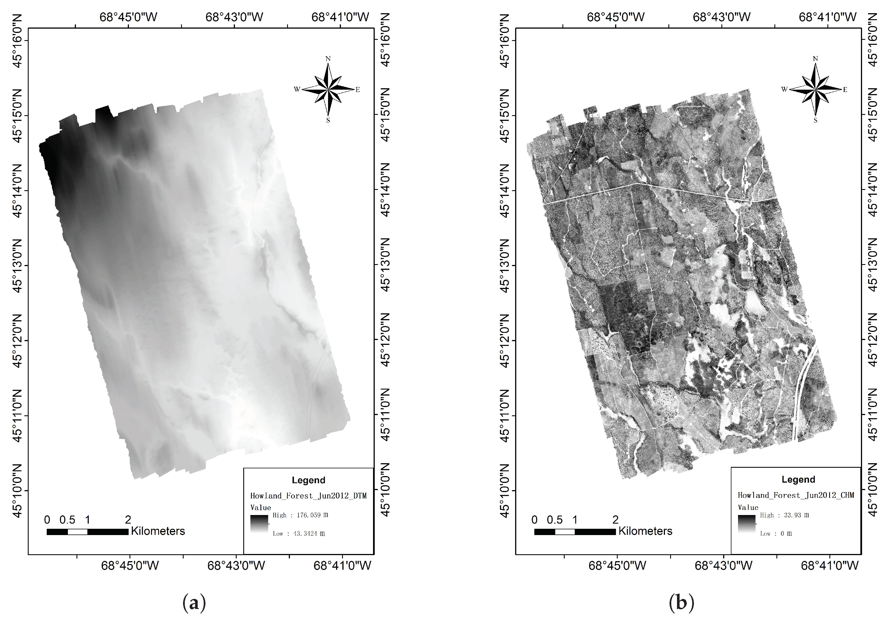
2.3. Airborne LiDAR Data from G-LiHT

The airborne small footprint LiDAR data from G-LiHT was collected in June 2012, which is near the acquisition time of the SIMPL data. G-LiHT is a portable, airborne imaging system that simultaneously maps the composition, structure, and function of terrestrial ecosystems using a combination of LiDAR, Hyperspectral, and Thermal sensors. G-LiHT’s profiling LiDAR is an LD321-A40 (Riegl USA, Orlando, FL, USA), multi-purpose laser distance meter which produces a 50 cm diameter footprint at the nominal operating altitude of 335 m [38]. Figure 3a,b shows the 1 m resolution Digital Terrain Model (DTM) and the Canopy Height Model (CHM) driven from the point cloud of G-LiHT.

2.4. Field Measurement
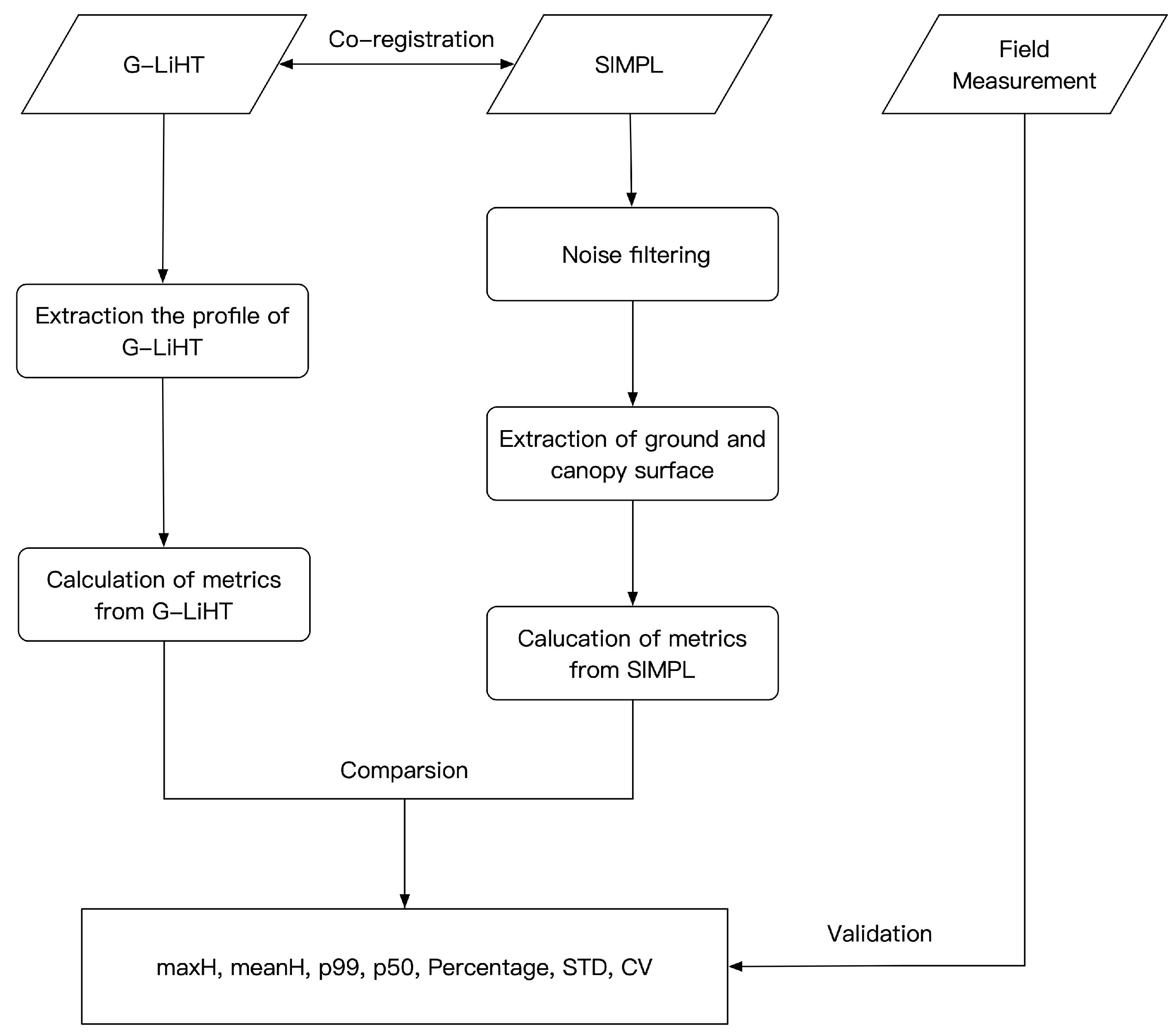
The stem map was collected in the year 2010. There is a total number of 7989 trees at a rectangle size of 150 m × 200 m. The field measurements include tree species, tree height, diameter at breast height (DBH), crown diameter at North-South direction (d-North-South) and crown diameter at East-West direction (d-East-West), which are summarized in Table 1.

3. Methods

3.1. Overview

The method we use in this study is shown in Figure 4. The method is divided into 4 parts: first, we extract the ground and canopy surface from the potential signal photons identified by the noise filtering algorithm using a local outlier factor (LOF) with an elliptical searching area [39]. Next, a co-registration technique based on moving profiling is applied between SIMPL data and G-LiHT data to correct the geolocation error. Then, we calculate the height metrics from both photon counting LiDAR data from SIMPL and airborne small footprint LiDAR data from G-LiHT. Finally, we investigate the relationship between the two sets of metrics, and use the stem map from field measurement to validate the results.

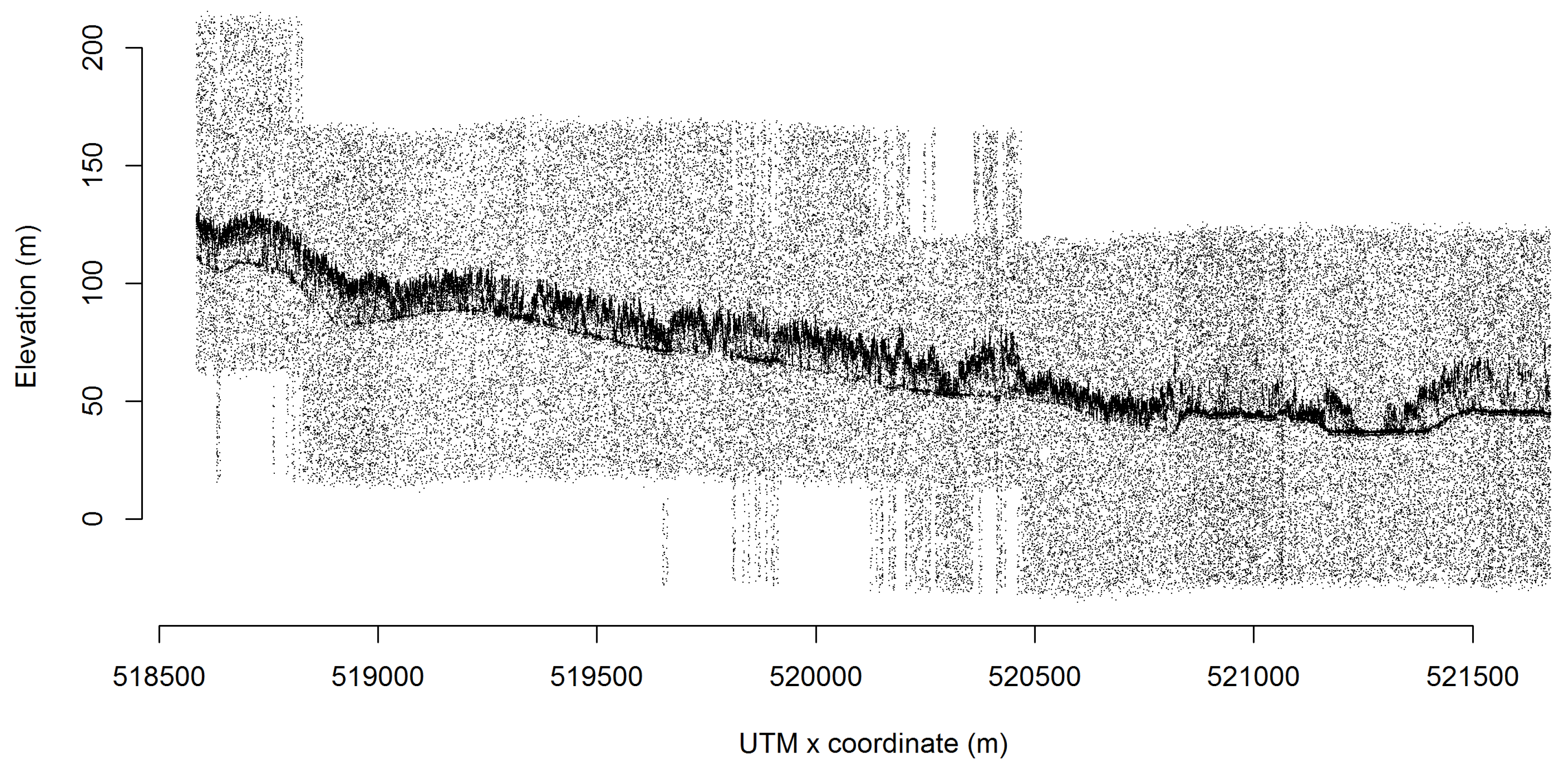
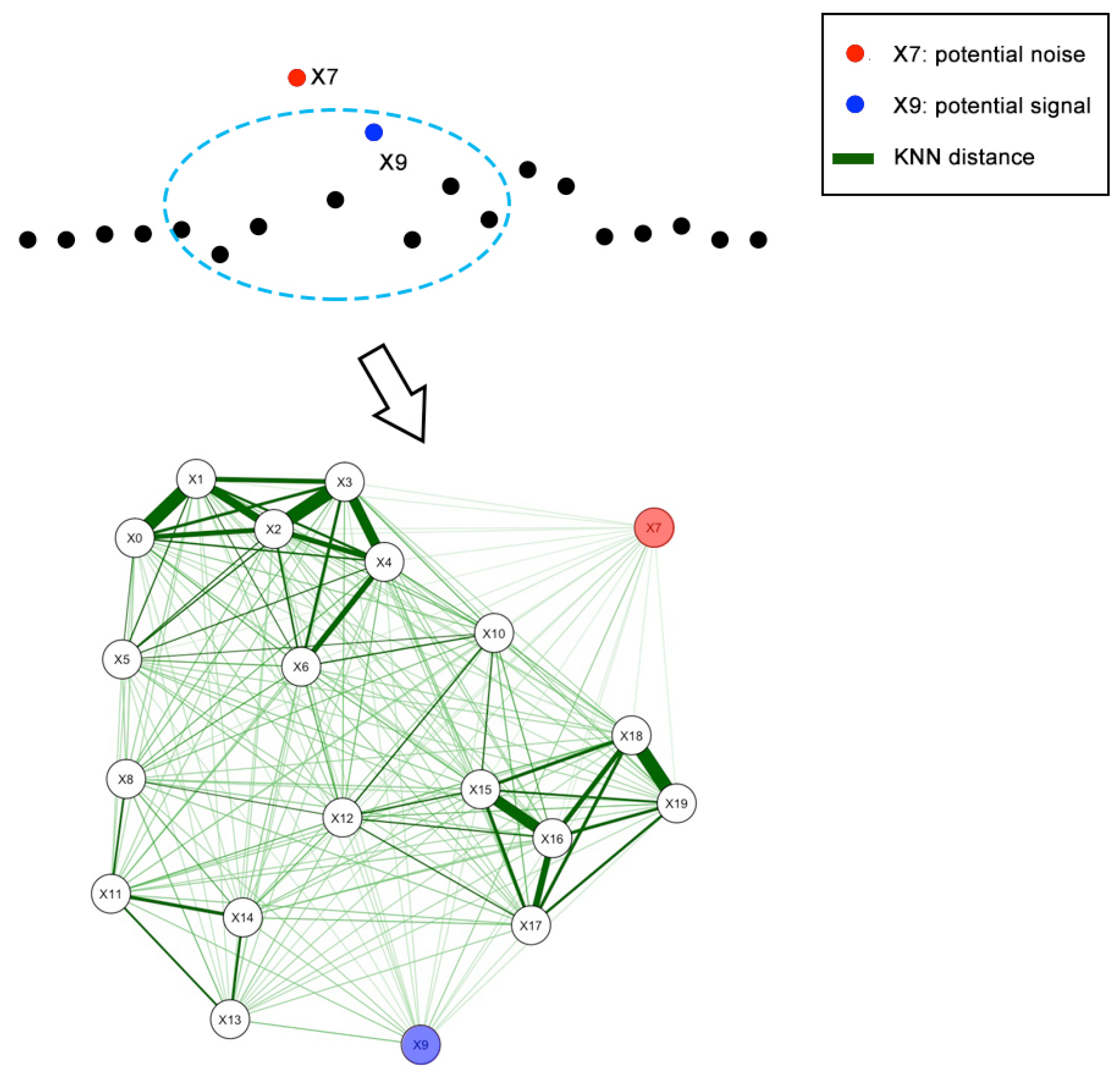
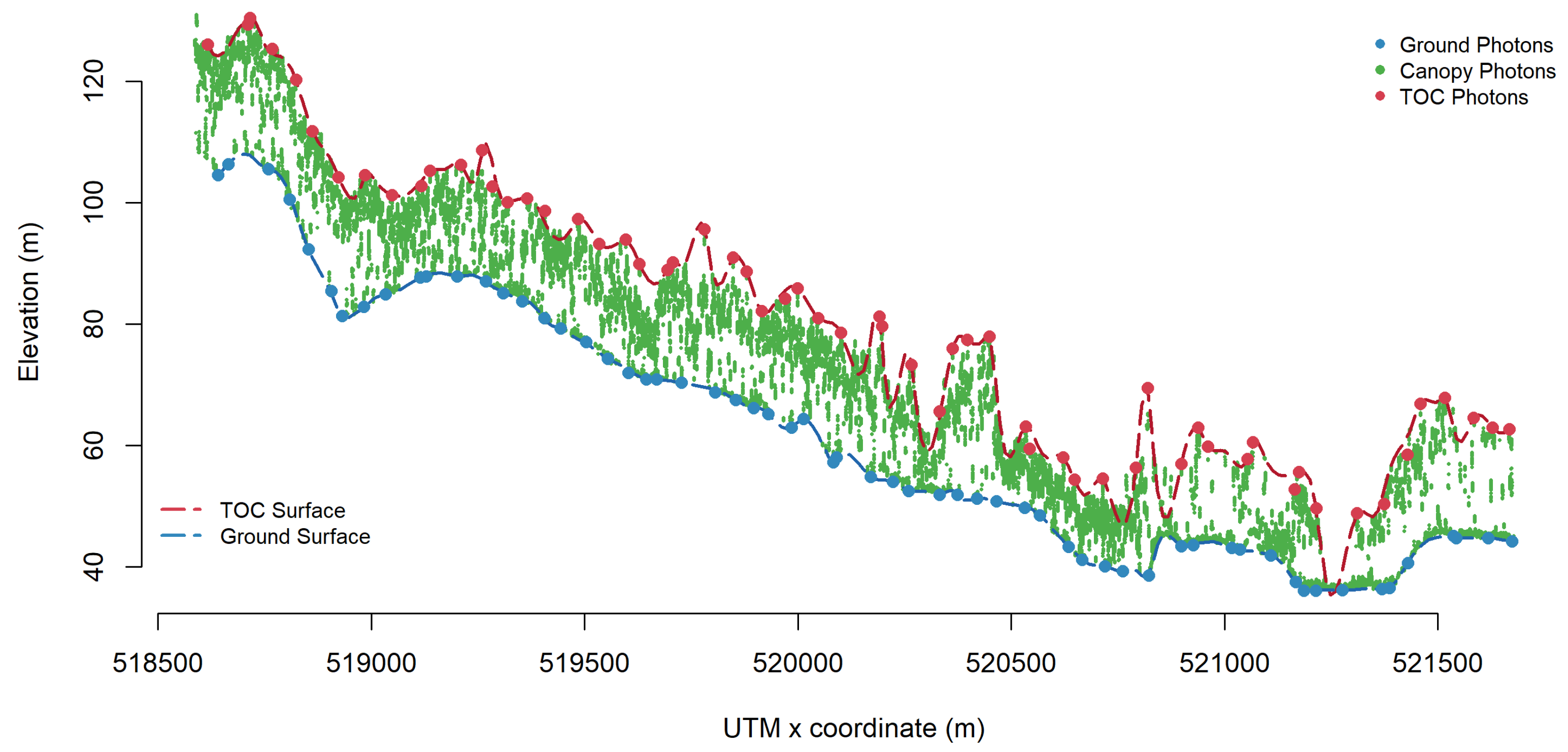
3.2. Extraction of Ground and Canopy Surface

It can be seen from Figure 2 that there are abundant noise photons with apparent locations ranging from the atmosphere to below ground level, which makes it difficult to detect vegetation and ground photons with existing methods that work on airborne point cloud data. However, it is still noticeable that the density of the signal photons is different in terms of horizontal and vertical directions, therefore we implement a modified LOF algorithm with an elliptical search area and assign the class tag based on the score which was returned.
LOF is an unsupervised outlier detection method which computes a score for a point which indicates the local density around the given point to its near neighbors [40]. The outliers are considered to be the points which are substantially lower than a threshold score compared with the density level among their neighbors.
For the noise detection method we propose here, we first calculate the K-Nearest Neighbors (KNN) distance using an elliptical search area for every photon. For any given point p and q in the data, the elliptical search area is defined by the following equation:
d i s t k ( p , q ) = ( x p x q ) 2 a 2 + ( h p h q ) 2 b 2
where x and h represent the distance and height of photons, a and b represent the major and minor axis of the ellipse respectively. In this paper, we use an empirical ratio which is a:b = 6:1 [39].
Figure 5 demonstrates the distance matrix from the ellipse searching shape. The red dot stands for point X7 and the blue dot stands for point X9. It can be seen from the figure that for a horizontal ellipse searching area, the potential noise point X7 can be distinguished from the signal point X9.
Next, a reachability distance from point p to q is estimated using Equation (2), which is the maximum value between the KNN distance of point q and the distance from point p and q. Then a reachability distance function of each point from its neighbors is calculated to get a local reachability density function.
r e a c h d i s t ( p , q ) = max { ( d i s t k ( q ) , d i s t ( p , q ) }
Furthermore, we will get the score of the local outlier factor with the ellipse nearest neighbors, which is defined as the average local reachability density of the neighbors divided by point p’s own local reachability density. If this score is greater than the mean value of scores then it is classified as signal otherwise as noise. Although most of the noise can be removed by filtering the higher LOF scores, there can still be some dense cluster centers within the noise photons. To correct the mislabeling points, a histogram filter was implemented to detect these noise photons. In addition, we used a moving window to find the local maximum and minimum value within the signal photons as the top of canopy (TOC) and ground seed points respectively. Finally, cubic spline interpolation is used to get the canopy and ground surface.

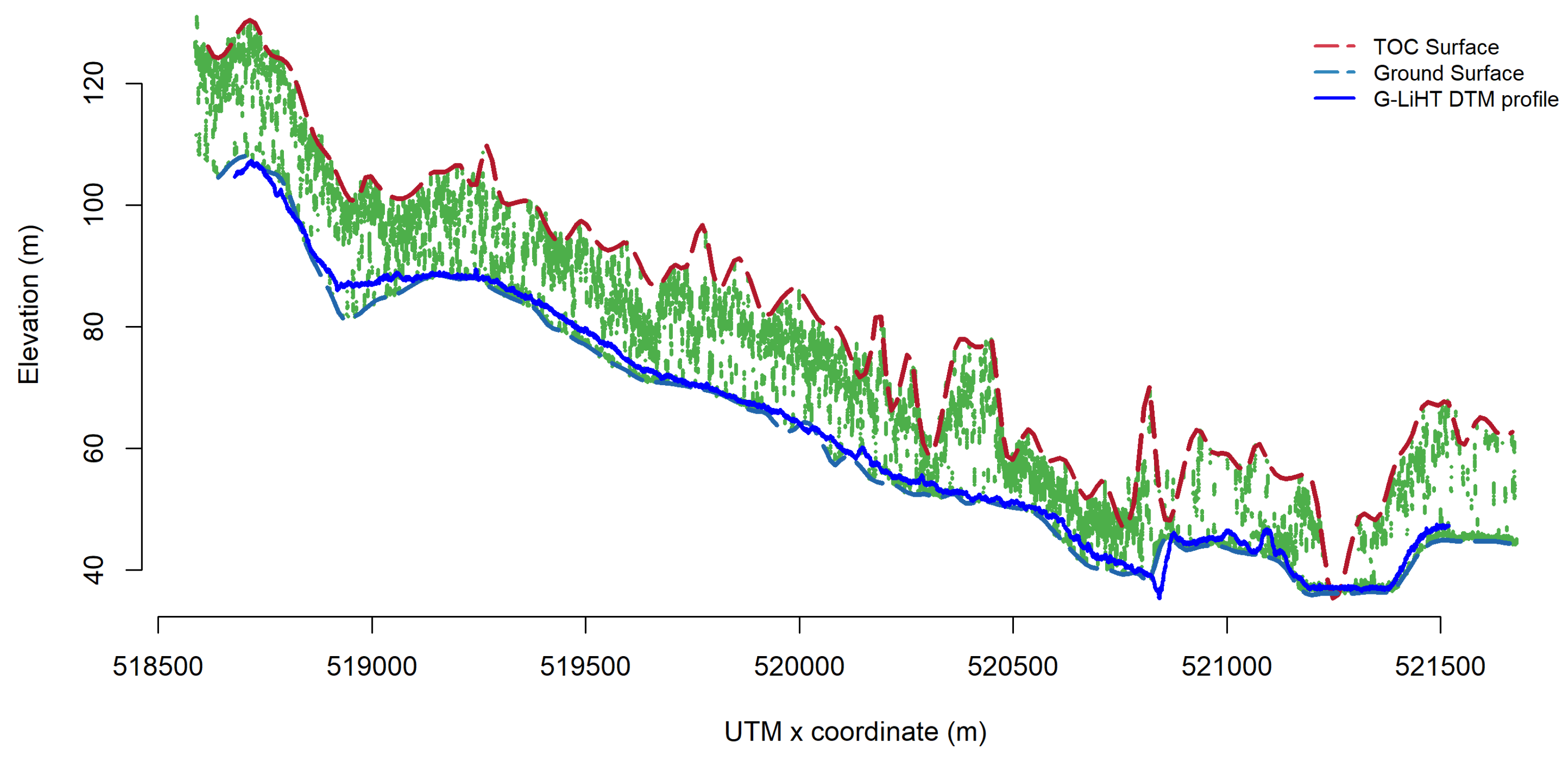
3.3. Co-Registration between SIMPL and G-LiHT Data

It can be seen that the geolocation between the SIMPL and G-LiHT data is not satisfying; therefore, an approach based on moving profiling [28] is implemented to match these two datasets. First, we extract the ground photons from our signal detection results and create a DTM profile; next we compare this profile with the DTM profile generated from G-LiHT. Then we shift the X-Y coordinates of the SIMPL-DTM profile, tracking the RMSE in the difference between these two profiles. Finally, the shift that produces the minimum RMSE is then considered to be the least error position, thus we add that shift to the SIMPL photons’ coordinates to obtain the corrected geolocation.

3.4. Metrics and Accuracy Assessment

Table 2 shows the 14 height metrics from the 2 groups that we used in this study. The metrics from photon counting LiDAR data are calculated based on similar concepts from the traditional point cloud LiDAR metrics such as height statistics and fractions. Height statistics include the maxH, meanH, height percentiles, standard deviation (STD) and coefficient of variation (CV), which are considered to have good relationships with forest height. In addition, the fraction of the number of points/photons above 1.3 m is considered to be a good indicator of forest canopy cover.
In addition, 6 different scale sizes ranging from 10 m to 50 m are designed to investigate the suitable statistical size to estimate relevant forest parameters for the forest application of ICESat-2 data, of which the 16 m value is the nominal footprint size for ICESat-2. Also, the nominal along-track sampling distance is 0.7 m, resulting in very dense overlapping footprints along the trajectory, which would be useful to aggregate all these observations to form some certain link-scale sizes for the parameter inversion. Therefore, we designed a few sizes from 10 m up to 50 m, given that SIMPL has a similar design like ATLAS.
To assess the accuracy of the results for these two datasets and the field measurement, four statistical indicators known as coefficient of determination ( R 2 ), Root Mean Square Error (RMSE), relative RMSE (rRMSE), and relative Error (rError) are computed to conduct the validation, where rRMSE and rError are defined as follows:
r R M S E = R M S E y i ¯ × 100 %
r E r r o r = y i y i y i × 100 %
where y i stands for the metrics from the reference value for the ith observation; y i ¯ is the mean value of y i ; y i are the metrics from the photon counting LiDAR data for the ith observation.

4. Results

4.1. Results of Extraction of Ground and Canopy Surface

The result of forest signal detection from SIMPL data is shown in Figure 6. It can be seen from the result that our method can separate the forest signal from the noise effectively. The photons which belong to the TOC, ground and within the canopy are well detected, especially in a quite high noise rate environment in relatively rough terrain across our study site. It is also noticeable that the TOC surface and ground surface are extracted accurately.

4.2. Results of Co-Registration between SIMPL and G-LiHT Data

Figure 7 demonstrates the result of the moving profiling method to match the SIMPL and G-LiHT data. The red dash line represents the TOC surface; the grey dash line represents the ground surface, and the blue line represents the best fitting G-LiHT DTM profile, which is considered to be the shift that produced the minimum RMSE between the SIMPL and G-LiHT DTM profile. It can be seen that with the correction of the geolocation, the co-registration between SIMPL and G-LiHT data has been improved.

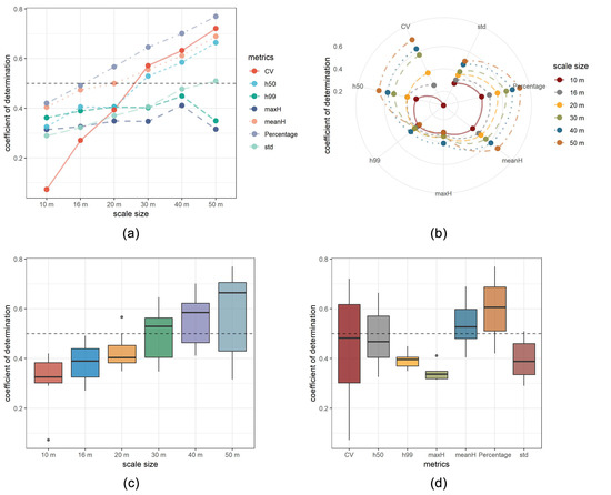
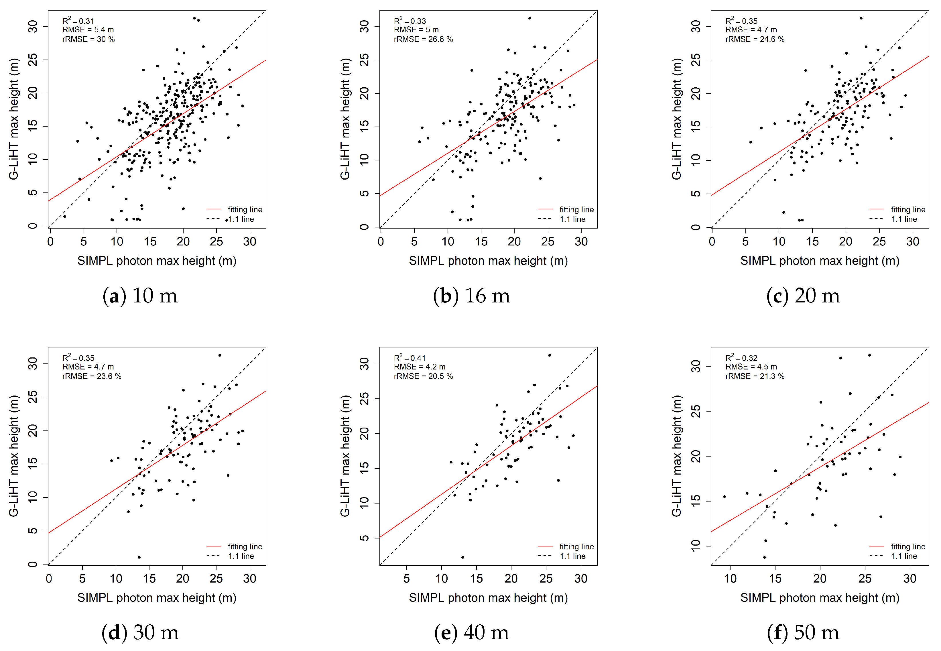
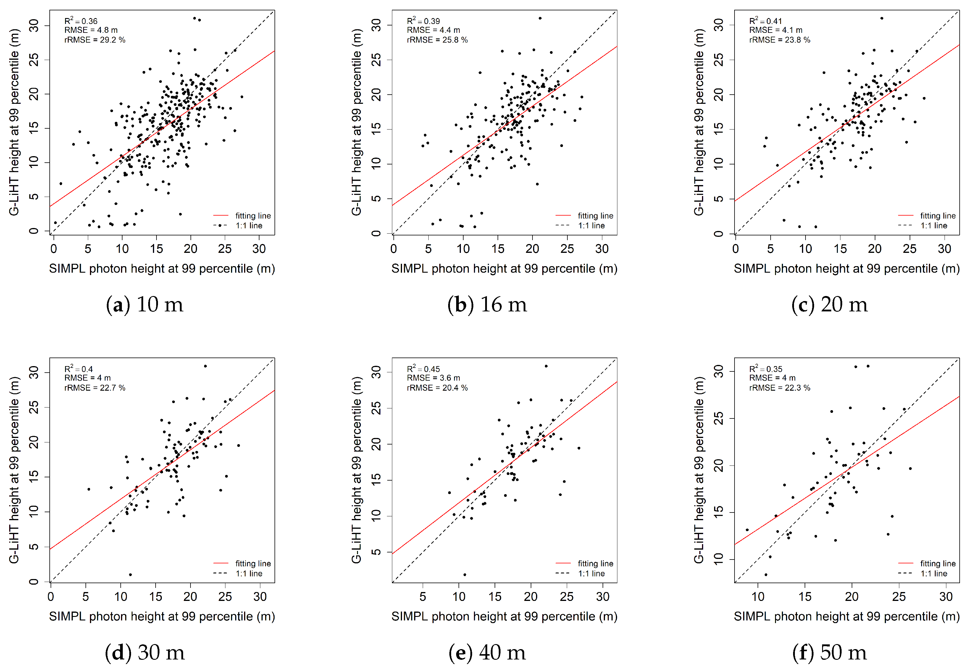
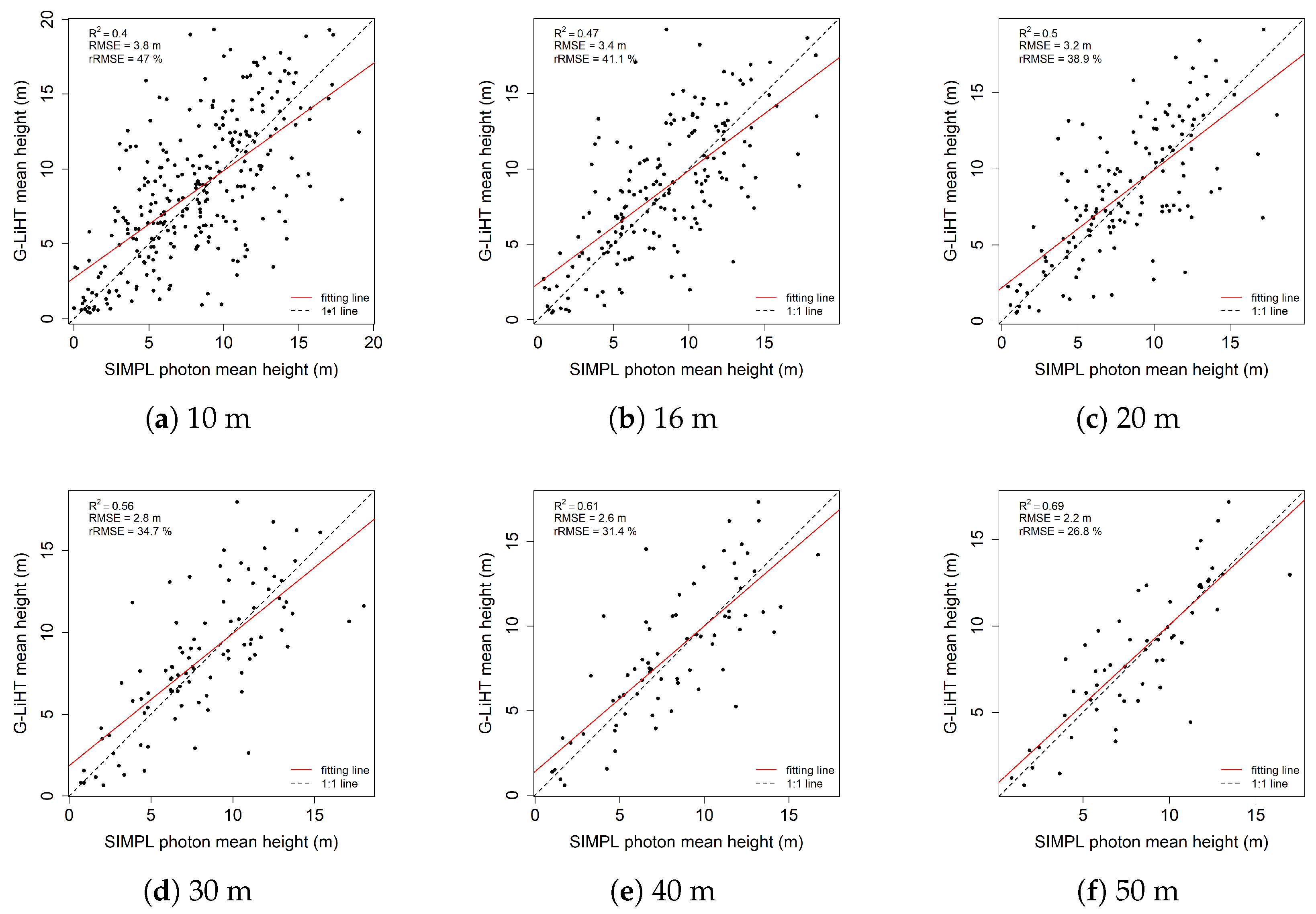
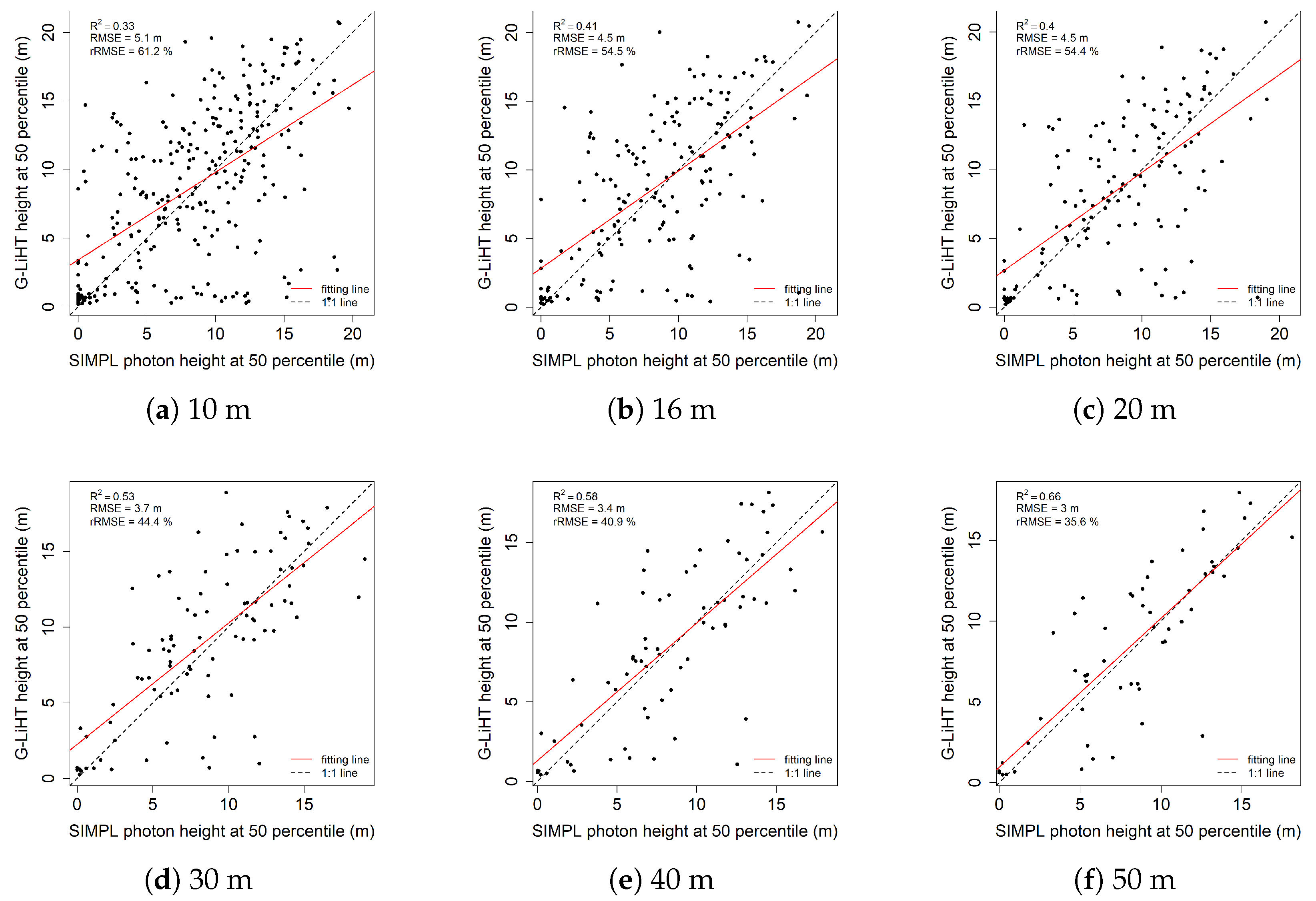
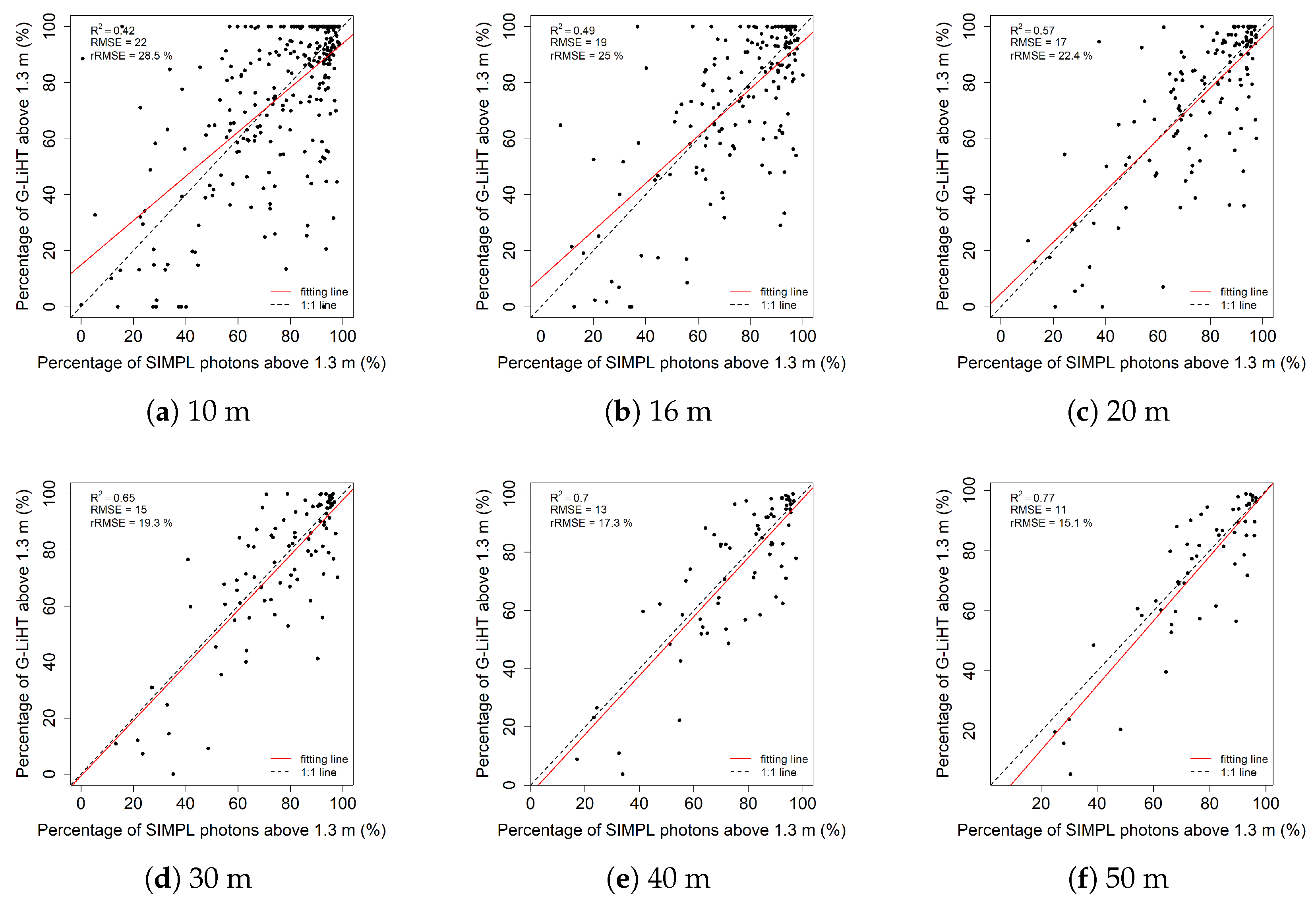
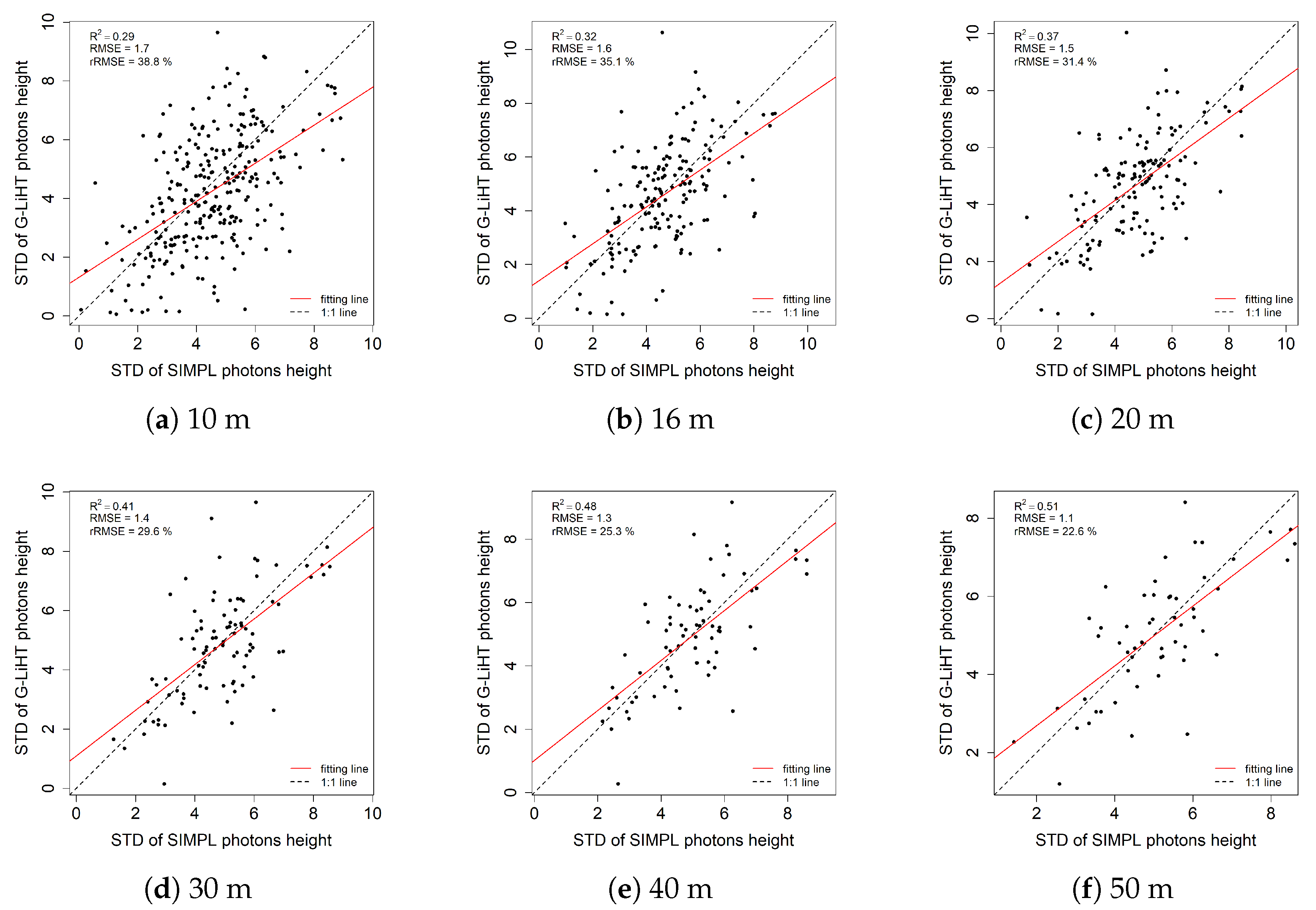
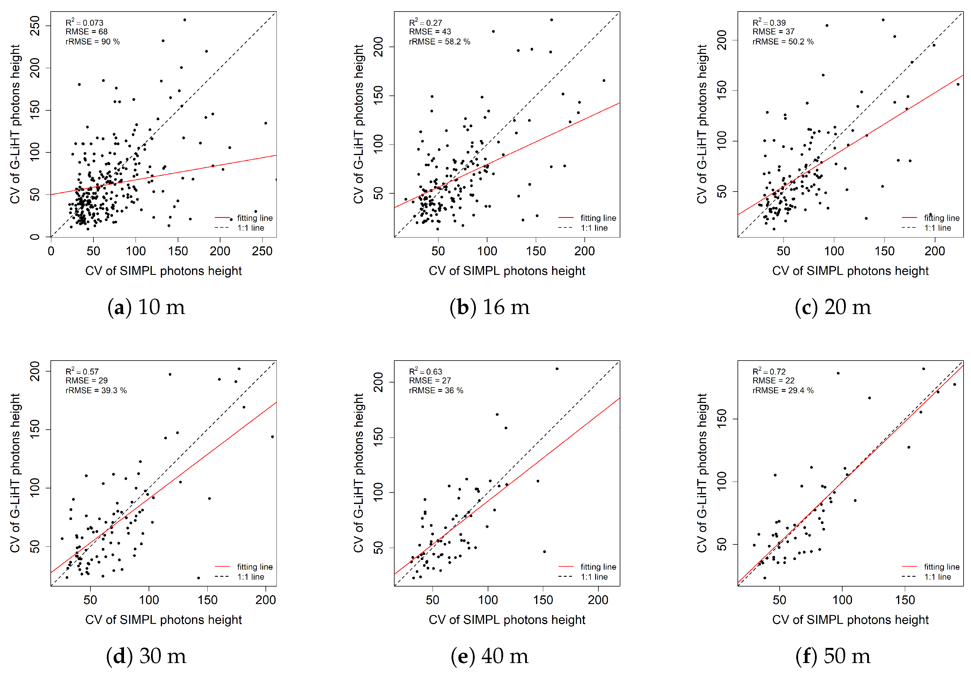
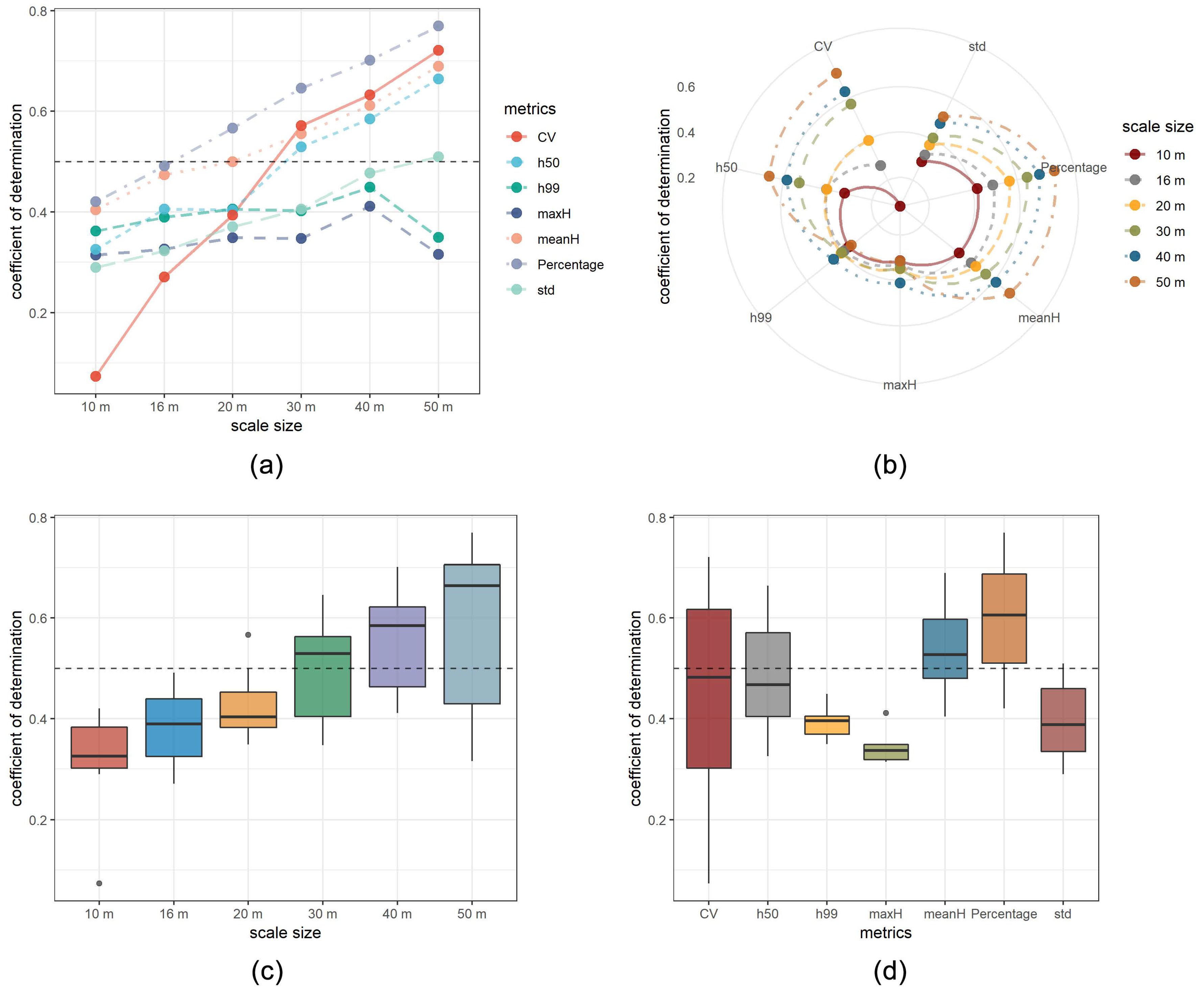
4.3. Results of Metrics from SIMPL Data

For the analysis of photon counting LiDAR metrics from the SIMPL data, we compared the relationship of the metrics including the maxH, meanH, height percentiles, standard deviation (STD), coefficient of variation (CV) and fraction of the number of points/photons above 1.3 m, from the relevant metrics derived from SIMPL and G-LiHT data. Here we investigate 6 different scales ranging from 10 m to 50 m, of which the 16 m value is the nominal footprint size for the ICESat-2 mission.
The results of the max tree height related metrics from SIMPL data show good consistency with those from G-LiHT. Figure 8 shows the relationship between the max value of all photon heights from SIMPL and the max value of all return heights from G-LiHT for different scales. It can be seen from these figures that the 40 m scale has the highest value of R-square and the lowest value of RMSE. In terms of the results of max height, Figure 9 shows similar findings for the 99th height percentile. The mean R-square values for all these six different scale sizes are 0.35 and 0.39 for the max value of height and the 99th height percentile respectively. The 99th height percentile has a slightly higher overall accuracy over the max height metrics with an increasing percentage of 3–6%. The mean value of the RMSE for the max values of height and the 99th height percentile are 4.8 m and 4.2 m respectively, which shows a difference which is over 4 m for the estimation of max tree height in our study site.
The results of mean tree height related metrics including the 50th height percentile and mean value of heights are shown in Figure 10 and Figure 11. The mean R-square values for all these six different scale sizes are 0.54 and 0.49 for the mean value of height and the 50th height percentile respectively. It shows that the overall accuracy to estimate mean tree height for the different scales is better than those of max tree height metrics with improvements of 19% and 10% respectively. Also, we can see the mean height metric has a higher overall accuracy compared with the 50th height percentile, with an increasing percentage of 3–10% for the different scale sizes. Compared with metrics related to the max tree height, the mean values of the RMSE for the mean value of height and the 50th height percentile are 3 m and 4 m respectively, of which the best fitting result is at the scale size of 50 m with an R-square of 0.69 and RMSE of 2.2 m for the mean value of height. It is also noticeable that with a smaller scale size, the range of the rRMSE values of meanH is 26.8–47% compared with those values of 21.3–30% from maxH, suggesting that the maxH maintains relatively good estimation for small scale sizes.
The fraction of the number of photons above 1.3 m from SIMPL, which is considered to be related with the canopy cover, shows good consistency with the metrics from G-LiHT as demonstrated in Figure 12. The mean values of R-square and RMSE for all these six different scale sizes are 0.6 and 16% respectively, of which the best fitting result is for the 50 m scale size with an R-square over 0.6 and RMSE less than 15%.
Similarly, we investigate the consistency of the remaining two height metrics which are standard deviation (Figure 13) and coefficient of variation (Figure 14) of photon heights, which are indicators of the variability of the data. We find that the estimation accuracy for these two metrics increases with a larger scale size, especially for the coefficient of variation, where the R-square improved from 0.073 to 0.72.
To summarize, for the metrics related to the max tree height, we can see that the 99th height percentile have a higher overall accuracy over the max height metrics. However, it is also noticeable that the RMSE is over 4 m for the estimation. In terms of the metrics related to the mean tree height, it can be seen that the overall accuracy for the different scales is better than those of max tree height metrics. Also, we found that the RMSE dropped to around 2 m at the scale size of 50 m. Likewise, the statistical metrics like the standard deviation and coefficient of variation suggested similar patterns and the overall accuracy improves with a larger scale size. Finally, for all the metrics related to canopy cover, good results were achieved with a mean R-square of 0.6.

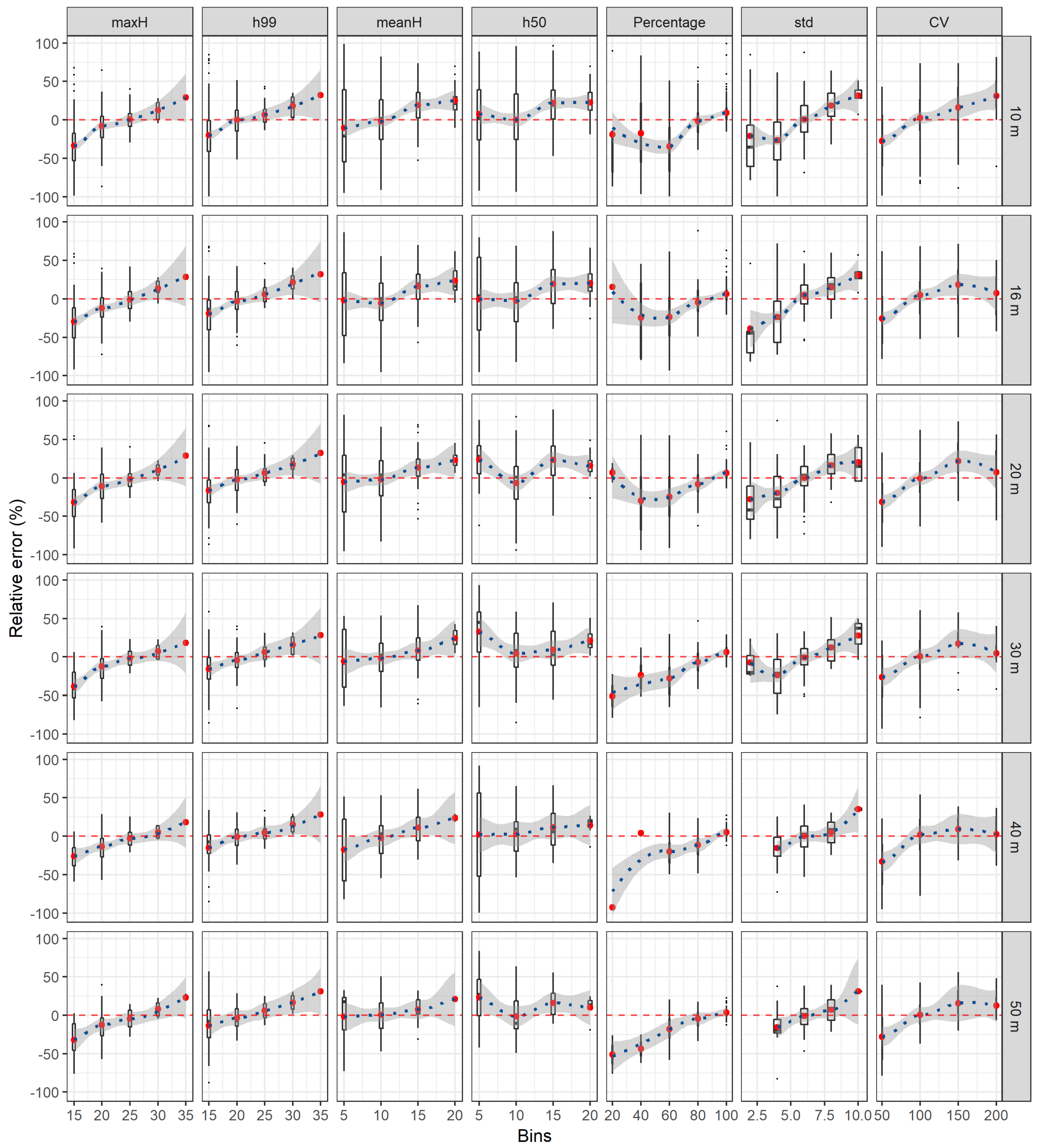
4.4. Validation with Field Measurements

To further investigate the potential of forest parameter estimation using photon counting LiDAR data, we use the stem map collected in the Howland Research Forest to validate the estimation accuracy of mean tree height from SIMPL data. As it is shown in Table 3, we compare both SIMPL and G-LiHT data at four different scale sizes ranging from 10 m to 30 m, and assess the results using three criteria including Mean Absolute Error (MAE), Standard Deviation (SD) and Root Mean Square Error (RMSE). Since the trajectory across our plot is less than 200 m, we only analyze scale sizes of up to 30 m.
The results from Table 3 suggest that the geolocation corrected G-LiHT data has a relatively good consistency with our field measurements, with mean values of 2.1 m, 2.4 m and 2.4 m for MAE, SD and RMSE respectively. For SIMPL data, the mean value of MAE is 2.9 m while the mean value of SD and RMSE are 5.3 m and 4.9 m.

5. Discussion

From the results of extraction of ground and canopy surfaces, we can see that the method we implemented using the local outlier factor modified with ellipse searching area achieved good results to detect the potential signal photons from the noise photons. The ellipse searching area utilized the unbalanced distribution of signal photons in the vertical direction compared with the original circle area of the local outlier factor detection algorithm, especially in a quite high noise rate environment in relatively rough terrain.
The ellipse searching area is determined by the ratio of the major and minor axis, the empirical ratio (a:b = 6:1) used for SIMPL data here is based on our previous testing results with 30 different MABEL/MATLAS data. Figure 15 shows the accuracy respond to various combinations of a and b. It can be seen from the figure that the four statistical indicators including accuracy, kappa coefficient, specificity, and F1, become stable at the ratio of 6:1. Although there is a small increase for specificity and F1 at the ratio of 8:1, the overall accuracy and kappa coefficient does not necessarily increase accordingly.
Furthermore, the detected photons which belong to the TOC, ground and within the canopy are also well depicted by the moving window technique. The canopy and ground surface extracted by applying the cubic spline interpolation showed good results in our study site. These results demonstrate that the noise filtering and surface extraction methods we implemented work well for SIMPL data in the Howland site, and could be potentially useful to extract forest photons from ICESat-2 data.
The results of co-registration between the SIMPL and G-LiHT data show that the geolocation problem between the SIMPL and G-LiHT data has been improved by extracting and examining the difference between these two profiles. In addition, validation results further confirmed the relatively good consistency from both the visual and statistical indicators. These findings proved that this moving profiling method would help to co-registration of the SIMPL and G-LiHT data, and could be further applied to match satellite data from ICESat-2 with other sources of remote sensing data. However, our method can only improve the relative matching result; we would expect to obtain a more accurate longitude–latitude geolocated photon set by introducing techniques like ground control points in the future.
The sensitivity analyses between the SIMPL and G-LiHT data in Howland site for different scale sizes are summarized in Figure 16. It can be seen that the coefficients of determination show clear increases with a larger scale size for most metrics. Interestingly, the max tree height related metrics (i.e., maxH and h99) do not necessarily give a better accuracy result with a larger scale size, where the R 2 dropped about 0.1 from 40 m to 50 m. The results also indicate that 40 m is the optimal scale size for estimating the max tree height with the highest value of R 2 and the lowest value of RMSE. In addition, it can be seen that h99 has better overall accuracy compared with maxH. One possible explanation is that the mechanism of the photon counting approach might miss hitting the very top of the canopy, resulting in the underestimation of the actual canopy profile. Another possible reason could be that some signal photons near the TOC were misidentified as noise photons, which would also likely add some uncertainty.
For the mean tree height related metrics (i.e., meanH and h50), the overall accuracies are higher than the max tree height related metrics in the same scale sizes, especially when the scale size is over 20 m. Also, we would expect a higher accuracy at the scale size of 50 m compared with other sizes, due to a relatively homogeneous forest type in our Howland site. However, it is also noticeable that there is a very small drop from 0.41 to 0.4 when the scale size increased from 16 m to 20 m for h50, suggesting that meanH has a better response than h50. Furthermore, the canopy cover related metrics (i.e., Percentage) also showed good relationships with the metrics from the G-LiHT data, which is likely because the forest closure is very high in the study site, as it can be seen that canopy cover cases which are over 80% contributed a large portion of all observations. Similarly, for the data variation related metrics (i.e., std and CV), we could expect a higher accuracy with a large scale size, since that more points would be included at a larger size, and there would be more likely the two datasets would show similar spatial distributions.
Furthermore, validation using the field measurements showed that the geolocation corrected G-LiHT profile has a relatively good consistency with field measurements compared with SIMPL. Although the mean absolute error of SIMPL is relatively low, the other two indicators show an error around 5 m. The possible explanation is that the SIMPL trajectory within our stem map is less than 200 m, resulting in a small number of observations especially for large scale sizes.
For optimal scale size, the line plot suggested that the best scale was not consistent across the various metrics, but observations from the boxplot indicated that there exists an increasing tendency, as the median value of accuracies for all metrics increased with a larger scale size. It is also noticeable that for scale sizes from 30 m to 50 m, the median values of accuracy are over 0.5, compared with around 0.4 for the scale size of 20 m, suggesting these would be relatively good statistical sizes for the estimation of forest parameters.
Theoretically, a large scale size would have better estimation results due to a more accurate profile is formed with more points been included, and most of the metrics indeed proved the best accuracy occurs at the size of 50 m. However, only for max tree height related metrics (i.e., maxH and h99), the optimal scale is 40 m rather than 50 m. To understand this inconsistency of these findings, we further analyze the relative error distribution of different bins for metrics at various scale sizes shown in Figure 17. These distributions are computed from the relative errors between the measurements from SIMPL and G-LiHT, and depicted with box-and-whisker plot overlaid with fitting lines, which are connected using the median values (center line) within each boxplot.
The distributions of relative errors within each bin size show variability that generally decreases from scale sizes of 10 m to 50 m. This variability is significant for the scale size of 10 to 30 m, especially for metrics such as Percentage, std, and CV. For these metrics, the one to one comparison for bins with lower values at smaller scales would more likely bring uncertainties due to fewer points come from photon counting LiDAR. Furthermore, the regression lines across the whole bins become increasingly linear, and the ’whiskers’ become shorter, indicating a tendency closer towards the center. In addition, it can be seen that the median value of the boxplot for height above 30 (35 in the graph) is closer to 0 at the size of 40 m, as well as the bins in the lower value side. This indicates that the size of 40 m has better estimations in the low and high tree heights, which could be more trees are included for the size of 50 m, and the dynamic range of the tree heights has been enlarged due to more trees are introduced with a larger scale size. However, this does not contribute a better estimation of maxH due to the photon counting approach. In the meantime, it brings some lower and higher values than the previous scale size, resulting in a potential loss of accuracy.
These findings are consistent with previous waveform LiDAR studies which showed that LVIS data (with a footprint size of 25 m in diameter) gives better estimation than GLAS data (with a footprint size of 70 m in diameter) [41,42]. It is also confirmed by simulation studies which prove the optimal footprint diameters of 25 and 30 m [43]. Also, study focus on MABEL data showed similar findings that 50 m is not always the optimal size to estimate the maxH [28].
The sensitivity studies showed the relatively good performance of the SIMPL data for dense conifer forest in our Howland site, but still it is not as good as the discrete return LiDAR system G-LiHT. We believe that better results could have been obtained if more accurately geolocated photons could be provided, despite the work we have done to match the SIMPL data. The SIMPL data used here is the Release 2 version, which is a preliminary work to produce geolocated SIMPL data in an HDF5 format. Also, the stability of the bias results within and between flights during a deployment has not been evaluated in detail, so the geolocated data are not considered to be fully calibrated. However, the 532 nm data from SIMPL is the same working wavelength as ATLAS, hence it is useful to inform methods for forest parameter estimation using ICESat-2 data.

6. Conclusions

This study implemented noise filtering and co-registration methods for SIMPL data at 532 nm, and further investigated the sensitivity of retrieval of forest parameters from SIMPL and G-LiHT data from a dense conifer forest in Howland for different scale sizes. The quantitative analyses and validation from the field measurements proved these metrics could contribute to the inputs of inversion models. We further found that h99 and meanH are good indicators for the estimation of max and mean tree height, and Percentage gives a good correspondence to describe canopy cover. In addition, std and CV both confirmed the similar spatial variations of these two datasets. We also found that the optimal scale size is around 50 m for the estimation of forest parameters. Results from the SIMPL data showed mean absolute error in height of 2–3 m, and fractional cover correlation with R 2 of 0.6. While more accurate results were possible with the dense spatial sampling of the discrete return G-LiHT, such dense sampling would not be available from satellite, and better estimations could be expected by integrating other sources of remote sensing data with the photon metrics we propose. These findings are of direct relevance to the estimation of forest parameters using photon counting LiDAR and could be of use for future applications of ICESat-2 vegetation studies.

Author Contributions

B.C. was responsible for the concept and methodology of the study as well as writing the manuscript. P.N. supported the methodology development and contributed to the writing process of the manuscript. Y.P. and Z.L. supported the concept development, provided important background information and contributed to the writing process of the manuscript, J.R., J.S. and I.B. provided much help for data collection and processing. G.S. and H.L. provided many helpful suggestions and comments for this manuscript.

Funding

This work was supported by the National Natural Science Foundation of China under Grant 41871278 and Grant 31570546, and the China Scholarship Council.

Acknowledgments

The authors would like to thank the ICESat-2 Project Science Office at NASA/GSFC for providing the photon counting LiDAR data used in this study. The authors would also like to thank the University of Maryland for providing the Howland forest stem map for this paper as the validation data. We also appreciate the valuable comments and constructive suggestions from the anonymous referees and the Academic Editor that helped improve the manuscript.

Conflicts of Interest

The authors declare no conflict of interest.

References

  1. Shevliakova, E.; Pacala, S.W.; Malyshev, S.; Hurtt, G.C.; Milly, P.; Caspersen, J.P.; Sentman, L.T.; Fisk, J.P.; Wirth, C.; Crevoisier, C. Carbon cycling under 300 years of land use change: Importance of the secondary vegetation sink. Glob. Biogeochem. Cycles 2009, 23. [Google Scholar] [CrossRef]
  2. Zolkos, S.G.; Goetz, S.J.; Dubayah, R. A meta-analysis of terrestrial aboveground biomass estimation using lidar remote sensing. Remote Sens. Environ. 2013, 128, 289–298. [Google Scholar] [CrossRef]
  3. Reese, H.; Nilsson, M.; Sandström, P.; Olsson, H. Applications using estimates of forest parameters derived from satellite and forest inventory data. Comput. Electron. Agric. 2002, 37, 37–55. [Google Scholar] [CrossRef]
  4. Kindermann, G.; McCallum, I.; Fritz, S.; Obersteiner, M. A global forest growing stock, biomass and carbon map based on FAO statistics. Silva Fennica 2008, 42, 387–396. [Google Scholar] [CrossRef]
  5. Fang, J.; Chen, A.; Peng, C.; Zhao, S.; Ci, L. Changes in forest biomass carbon storage in China between 1949 and 1998. Science 2001, 292, 2320–2322. [Google Scholar]
  6. Dubayah, R.O.; Drake, J.B. Lidar remote sensing for forestry. J. For. 2000, 98, 44–46. [Google Scholar]
  7. Koetz, B.; Morsdorf, F.; Sun, G.; Ranson, K.J.; Itten, K.; Allgower, B. Inversion of a lidar waveform model for forest biophysical parameter estimation. IEEE Geosci. Remote Sens. Lett. 2006, 3, 49–53. [Google Scholar] [CrossRef]
  8. Rosette, J.; Suárez, J.; North, P.; Los, S. Forestry applications for satellite LiDAR remote sensing. Photogramm. Eng. Remote Sens. 2011, 77, 271–279. [Google Scholar] [CrossRef]
  9. Rosette, J.; Cook, B.; Nelson, R.; Huang, C.; Masek, J.; Tucker, C.; Sun, G.; Huang, W.; Montesano, P.; Rubio-Gil, J.; et al. Sensor Compatibility for Biomass Change Estimation Using Remote Sensing Data Sets: Part of NASA’s Carbon Monitoring System Initiative. IEEE Geosci. Remote Sens. Lett. 2015, 12, 1511–1515. [Google Scholar] [CrossRef]
  10. Lefsky, M.A.; Harding, D.J.; Keller, M.; Cohen, W.B.; Carabajal, C.C.; Del Bom Espirito-Santo, F.; Hunter, M.O.; de Oliveira, R. Estimates of forest canopy height and aboveground biomass using ICESat. Geophys. Res. Lett. 2005, 32, L22S02. [Google Scholar] [CrossRef]
  11. Keller, M. Revised method for forest canopy height estimation from Geoscience Laser Altimeter System waveforms. J. Appl. Remote Sens. 2007, 1, 013537. [Google Scholar] [CrossRef]
  12. Duncanson, L.I.; Niemann, K.O.; Wulder, M.A. Estimating forest canopy height and terrain relief from GLAS waveform metrics. Remote Sens. Environ. 2010, 114, 138–154. [Google Scholar] [CrossRef]
  13. Bye, I.; North, P.R.; Los, S.; Kljun, N.; Rosette, J.; Hopkinson, C.; Chasmer, L.; Mahoney, C. Estimating forest canopy parameters from satellite waveform LiDAR by inversion of the FLIGHT three-dimensional radiative transfer model. Remote Sens. Environ. 2017, 188, 177–189. [Google Scholar] [CrossRef]
  14. Lefsky, M.; Keller, M.; Harding, D.; Pang, Y. A Global Forest Canopy Height and Vertical Structure Product from the Geoscience Laser Altimeter System. In AGU Fall Meeting Abstracts; American Geophysical Union: San Francisco, CA, USA, 2006. [Google Scholar]
  15. Los, S.; Rosette, J.; Kljun, N.; North, P.; Chasmer, L.; Suárez, J.; Hopkinson, C.; Hill, R.; Van Gorsel, E.; Mahoney, C.; et al. Vegetation height products between 60 S and 60 N from ICESat GLAS data. Geosci. Model Dev. 2012, 5, 413–432. [Google Scholar] [CrossRef]
  16. Markus, T.; Neumann, T.; Martino, A.; Abdalati, W.; Brunt, K.; Csatho, B.; Farrell, S.; Fricker, H.; Gardner, A.; Harding, D.; et al. The Ice, Cloud, and land Elevation Satellite-2 (ICESat-2): Science requirements, concept, and implementation. Remote Sens. Environ. 2017, 190, 260–273. [Google Scholar] [CrossRef]
  17. Leigh, H.W.; Magruder, L.A.; Carabajal, C.C.; Saba, J.L.; McGarry, J.F. Development of Onboard Digital Elevation and Relief Databases for ICESat-2. IEEE Trans. Geosci. Remote Sens. 2015, 53, 2011–2020. [Google Scholar] [CrossRef]
  18. Troupaki, E.; Denny, Z.H.; Wu, S.; Bradshaw, H.N.; Smith, K.A.; Hults, J.A.; Ramos-Izquierdo, L.A.; Cook, W.B. Space qualification of the optical filter assemblies for the ICESat-2/ATLAS instrument. In Proceedings of the Components and Packaging for Laser Systems. International Society for Optics and Photonics, San Francisco, CA, USA, 20 February 2015; Volume 9346, p. 93460H. [Google Scholar]
  19. Anthony, W.Y.; Harding, D.J.; Dabney, P.W. Laser transmitter design and performance for the slope imaging multi-polarization photon-counting lidar (SIMPL) instrument. In Proceedings of the Solid State Lasers XXV: Technology and Devices. International Society for Optics and Photonics, San Francisco, CA, USA, 16 March 2016; Volume 9726, p. 97260J. [Google Scholar]
  20. Brunt, K.; Neumann, T.; Markus, T.; Cook, W.; Hart, W.; Webb, C.; Dimarzio, J.; Hancock, D.; Lee, J.; Bhardwaj, S.; et al. MABEL photon-counting altimetry data for ICESat-2 simulations. In AGU Fall Meeting Abstracts; American Geophysical Union: San Francisco, CA, USA, 2011. [Google Scholar]
  21. McGill, M.; Markus, T.; Scott, S.S.; Neumann, T. The multiple altimeter beam experimental lidar (MABEL): An airborne simulator for the ICESat-2 mission. J. Atmos. Ocean. Technol. 2013, 30, 345–352. [Google Scholar] [CrossRef]
  22. Brunt, K.M.; Neumann, T.A.; Amundson, J.M.; Kavanaugh, J.L.; Moussavi, M.S.; Walsh, K.M.; Cook, W.B.; Markus, T. MABEL photon-counting laser altimetry data in Alaska for ICESat-2 simulations and development. Cryosphere 2016, 10. [Google Scholar] [CrossRef]
  23. Rosette, J.; Field, C.; Nelson, R.; Decola, P.; Cook, B.; Degnan, J. Single-Photon LiDAR for Vegetation Analysis. In AGU Fall Meeting Abstracts; American Geophysical Union: San Francisco, CA, USA, 2011. [Google Scholar]
  24. Magruder, L.A.; Brunt, K.M. Performance Analysis of Airborne Photon-Counting Lidar Data in Preparation for the ICESat-2 Mission. IEEE Trans. Geosci. Remote Sens. 2018, 56, 2911–2918. [Google Scholar] [CrossRef]
  25. Brunt, K.M.; Neumann, T.A.; Walsh, K.M.; Markus, T. Determination of Local Slope on the Greenland Ice Sheet Using a Multibeam Photon-Counting Lidar in Preparation for the ICESat-2 Mission. IEEE Geosci. Remote Sens. Lett. 2014, 11, 935–939. [Google Scholar] [CrossRef]
  26. Herzfeld, U.C.; McDonald, B.W.; Wallin, B.F.; Neumann, T.A.; Markus, T.; Brenner, A.; Field, C. Algorithm for Detection of Ground and Canopy Cover in Micropulse Photon-Counting Lidar Altimeter Data in Preparation for the ICESat-2 Mission. IEEE Trans. Geosci. Remote Sens. 2014, 52, 2109–2125. [Google Scholar] [CrossRef]
  27. Zhang, J.; Kerekes, J. An Adaptive Density-Based Model for Extracting Surface Returns from Photon-Counting Laser Altimeter Data. IEEE Geosci. Remote Sens. Lett. 2015, 12, 726–730. [Google Scholar] [CrossRef]
  28. Gwenzi, D.; Lefsky, M.A.; Suchdeo, V.P.; Harding, D.J. Prospects of the ICESat-2 laser altimetry mission for savanna ecosystem structural studies based on airborne simulation data. ISPRS J. Photogramm. Remote Sens. 2016, 118, 68–82. [Google Scholar] [CrossRef]
  29. Popescu, S.; Zhou, T.; Nelson, R.; Neuenschwander, A.; Sheridan, R.; Narine, L.; Walsh, K. Photon counting LiDAR: An adaptive ground and canopy height retrieval algorithm for ICESat-2 data. Remote Sens. Environ. 2018, 208, 154–170. [Google Scholar] [CrossRef]
  30. Brown, M.E.; Arias, S.D.; Neumann, T.; Jasinski, M.F.; Posey, P.; Babonis, G.; Glenn, N.F.; Birkett, C.M.; Escobar, V.M.; Markus, T. Applications for ICESat-2 Data: From NASA’s Early Adopter Program. IEEE Geosci. Remote Sens. Mag. 2016, 4, 24–37. [Google Scholar] [CrossRef]
  31. Neuenschwander, A.L.; Magruder, L.A. The potential impact of vertical sampling uncertainty on ICESat-2/ATLAS terrain and canopy height retrievals for multiple ecosystems. Remote Sens. 2016, 8, 1039. [Google Scholar] [CrossRef]
  32. Swatantran, A.; Tang, H.; Barrett, T.; DeCola, P.; Dubayah, R. Rapid, high-resolution forest structure and terrain mapping over large areas using single photon lidar. Sci. Rep. 2016, 6, 28277. [Google Scholar] [CrossRef]
  33. Kwok, R.; Markus, T. Potential basin-scale estimates of Arctic snow depth with sea ice freeboards from CryoSat-2 and ICESat-2: An exploratory analysis. Adv. Space Res. 2017, 62, 1243–1250. [Google Scholar] [CrossRef]
  34. Glenn, N.F.; Neuenschwander, A.; Vierling, L.A.; Spaete, L.; Li, A.; Shinneman, D.J.; Pilliod, D.S.; Arkle, R.S.; McIlroy, S.K. Landsat 8 and ICESat-2: Performance and potential synergies for quantifying dryland ecosystem vegetation cover and biomass. Remote Sens. Environ. 2016, 185, 233–242. [Google Scholar] [CrossRef]
  35. Gwenzi, D.; Lefsky, M. Prospects of photon counting lidar for savanna ecosystem structural studies. In Proceedings of the International Archives of the Photogrammetry, Remote Sensing & Spatial Information Sciences, Denver, CO, USA, 7–20 November 2014. [Google Scholar]
  36. Nie, S.; Wang, C.; Xi, X.; Luo, S.; Li, G.; Tian, J.; Wang, H. Estimating the vegetation canopy height using micro-pulse photon-counting LiDAR data. Opt. Express 2018, 26, A520–A540. [Google Scholar] [CrossRef]
  37. Montesano, P.; Rosette, J.; Sun, G.; North, P.; Nelson, R.; Dubayah, R.; Ranson, K.; Kharuk, V. The uncertainty of biomass estimates from modeled ICESat-2 returns across a boreal forest gradient. Remote Sens. Environ. 2015, 158, 95–109. [Google Scholar] [CrossRef]
  38. Cook, B.D.; Corp, L.A.; Nelson, R.F.; Middleton, E.M.; Morton, D.C.; McCorkel, J.T.; Masek, J.G.; Ranson, K.J.; Ly, V.; Montesano, P.M. NASA Goddard’s LiDAR, hyperspectral and thermal (G-LiHT) airborne imager. Remote Sens. 2013, 5, 4045–4066. [Google Scholar] [CrossRef]
  39. Chen, B.; Pang, Y.; Li, Z.; Lu, H.; Liu, L.; North, P.; Rosette, J. Ground and Top of Canopy Extraction from Photon Counting LiDAR Data Using Local Outlier Factor with Ellipse Searching Area. IEEE Geosci. Remote Sens. Lett. 2019, in press. [Google Scholar] [CrossRef]
  40. Breunig, M.M.; Kriegel, H.P.; Ng, R.T.; Sander, J. LOF: Identifying density-based local outliers. Sigmod Record 2000, 29, 93–104. [Google Scholar] [CrossRef]
  41. Drake, J.B.; Dubayah, R.O.; Knox, R.G.; Clark, D.B.; Blair, J.B. Sensitivity of large-footprint lidar to canopy structure and biomass in a neotropical rainforest. Remote Sens. Environ. 2002, 81, 378–392. [Google Scholar] [CrossRef]
  42. Anderson, J.; Martin, M.; Smith, M.; Dubayah, R.; Hofton, M.; Hyde, P.; Peterson, B.; Blair, J.; Knox, R. The use of waveform lidar to measure northern temperate mixed conifer and deciduous forest structure in New Hampshire. Remote Sens. Environ. 2006, 105, 248–261. [Google Scholar] [CrossRef]
  43. Pang, Y.; Lefsky, M.; Sun, G.; Ranson, J. Impact of footprint diameter and off-nadir pointing on the precision of canopy height estimates from spaceborne lidar. Remote Sens. Environ. 2011, 115, 2798–2809. [Google Scholar] [CrossRef]
Figure 1. The location (right) of the Howland forest area, and image (left) of the Goddard’s LiDAR, Hyperspectral and Thermal Imager (G-LiHT) Canopy Height Model (CHM); the red line represents the SIMPL trajectory.
Remotesensing 11 00856 g001
Figure 2. The profile of the photon counting LiDAR data from SIMPL within the Howland Research Forest. The horizontal x-axis stands for the UTM x coordinate; the vertical y-axis stands for the ellipsoidal height.
Remotesensing 11 00856 g002
Figure 3. The 1 m resolution DTM and CHM of the study site driven from G-LiHT. (a) The DTM from G-LiHT. (b) The CHM from G-LiHT.
Remotesensing 11 00856 g003
Figure 4. The flowchart of the proposed method used in this study.
Remotesensing 11 00856 g004
Figure 5. The distance matrix from the horizontal ellipse searching area, a darker and thicker line indicates closer reachability between these points.
Remotesensing 11 00856 g005
Figure 6. The result of ground and canopy surface extraction in Howland research forest.
Remotesensing 11 00856 g006
Figure 7. The result of the moving profiling method to match the SIMPL and G-LiHT data.
Remotesensing 11 00856 g007
Figure 8. The relationship between the max value of all photon heights from SIMPL and the max value of all return heights from G-LiHT for different scales.
Remotesensing 11 00856 g008
Figure 9. The relationship between the 99th percentile of all photon heights from SIMPL and the 99th percentile of all return heights from G-LiHT for different scales.
Remotesensing 11 00856 g009
Figure 10. The relationship between the mean value of all photon heights from SIMPL and the mean value of all return heights from G-LiHT for different scales.
Remotesensing 11 00856 g010
Figure 11. The relationship between the 50th percentile of all photon heights from SIMPL and the 50th percentile of all return heights from G-LiHT for different scales.
Remotesensing 11 00856 g011
Figure 12. The relationship between the fraction of the number of photons above 1.3 m from SIMPL and the fraction of the number of points above 1.3 m from G-LiHT for different scales.
Remotesensing 11 00856 g012
Figure 13. The relationship between the standard deviation of all photon heights from SIMPL and the standard deviation of all return heights from G-LiHT for different scales.
Remotesensing 11 00856 g013
Figure 14. The relationship between the coefficient of variation of all photon heights from SIMPL and the coefficient of variation of all return heights from G-LiHT for different scales.
Remotesensing 11 00856 g014
Figure 15. The accuracy respond to different ratios of the ellipse searching area.
Remotesensing 11 00856 g015
Figure 16. The sensitivity analyses between the SIMPL and G-LiHT data in Howland site for different scale sizes.
Remotesensing 11 00856 g016
Figure 17. The relative error distribution of different bins for metrics at various scale sizes. The vertical y-axis represents the relative error (measurements from G-LiHT are used as reference values); the numbers in horizontal x-axis represent certain bin sizes. For example, in maxH graph, 15 stands for tree height within 0–15 m; 20 stands for 15–20 m; 25 stands for 20–25 m; 30 stands for 25–30 m; 35 stands for tree height above 30 m.
Remotesensing 11 00856 g017
Table 1. Statistics for the Howland stem map collected in 2010. Min is the minimum value, Max is the maximum value, Mean is the averaged value, and SD is the standard deviation.
SpeciesNo. of TreesStatisticsHeight (m)DBH (cm)d-East-West (m)d-North-South (m)
Hemlock7239Min3.172.900.211.10
Max37.9960.906.9113.21
Mean12.9412.121.194.5
SD7.918.100.532.75
Aspen750Min4.363.00.231.05
Max46.4761.82.6611.22
Mean15.4710.91.123.74
SD9.497.370.432.29
All7989Min3.172.90.211.05
Max46.4761.86.9113.21
Mean12.8312.01.194.43
SD7.868.040.522.72
Table 2. Height metrics from SIMPL and G-LiHT.
Source of DataName of the MetricsDescription
Metrics from SIMPLSmaxHMax value of all photon heights
SmeanHMean value of all photon heights
Sh9999th percentile of all photon heights
Sh5050th percentile of all photon heights
SPercentageFraction of the number of photons above 1.3 m
SSTDStandard deviation of all photon heights
SCVCoefficient of variation of all photon heights
Metrics from G-LiHTGmaxHMax value of all return heights
GmeanHMean value of all return heights
Gh9999th percentile of all return heights
Gh5050th percentile of all return heights
GPercentageFraction of the number of points above 1.3 m
GSTDStandard deviation of all return heights
GCVCoefficient of variation of all return heights
Table 3. Result of validation using the Howland stem map. MAE is mean absolute error, SD is the standard deviation, and RMSE is the root mean square error.
Data SourceScale SizeMAE (m)SD (m)RMSE (m)
G-LiHT10 m2.93.93.6
16 m2.41.72.1
20 m1.71.82.1
30 m1.22.11.9
Mean value2.12.42.4
SIMPL10 m3.54.64.5
16 m2.75.75.3
20 m35.45
30 m2.45.34.9
Mean value2.95.34.9

