The Use of Unmanned Aerial Systems to Map Intertidal Sediment


Zienkiewicz Centre for Computational Engineering, College of Engineering, Swansea University, Swansea SA1 8EN, UK
*
Author to whom correspondence should be addressed.
Remote Sens. 2018, 10(12), 1918; https://doi.org/10.3390/rs10121918
Submission received: 28 September 2018
/
Revised: 16 November 2018
/
Accepted: 26 November 2018
/
Published: 30 November 2018
(This article belongs to the Section Remote Sensing in Geology, Geomorphology and Hydrology)
Abstract
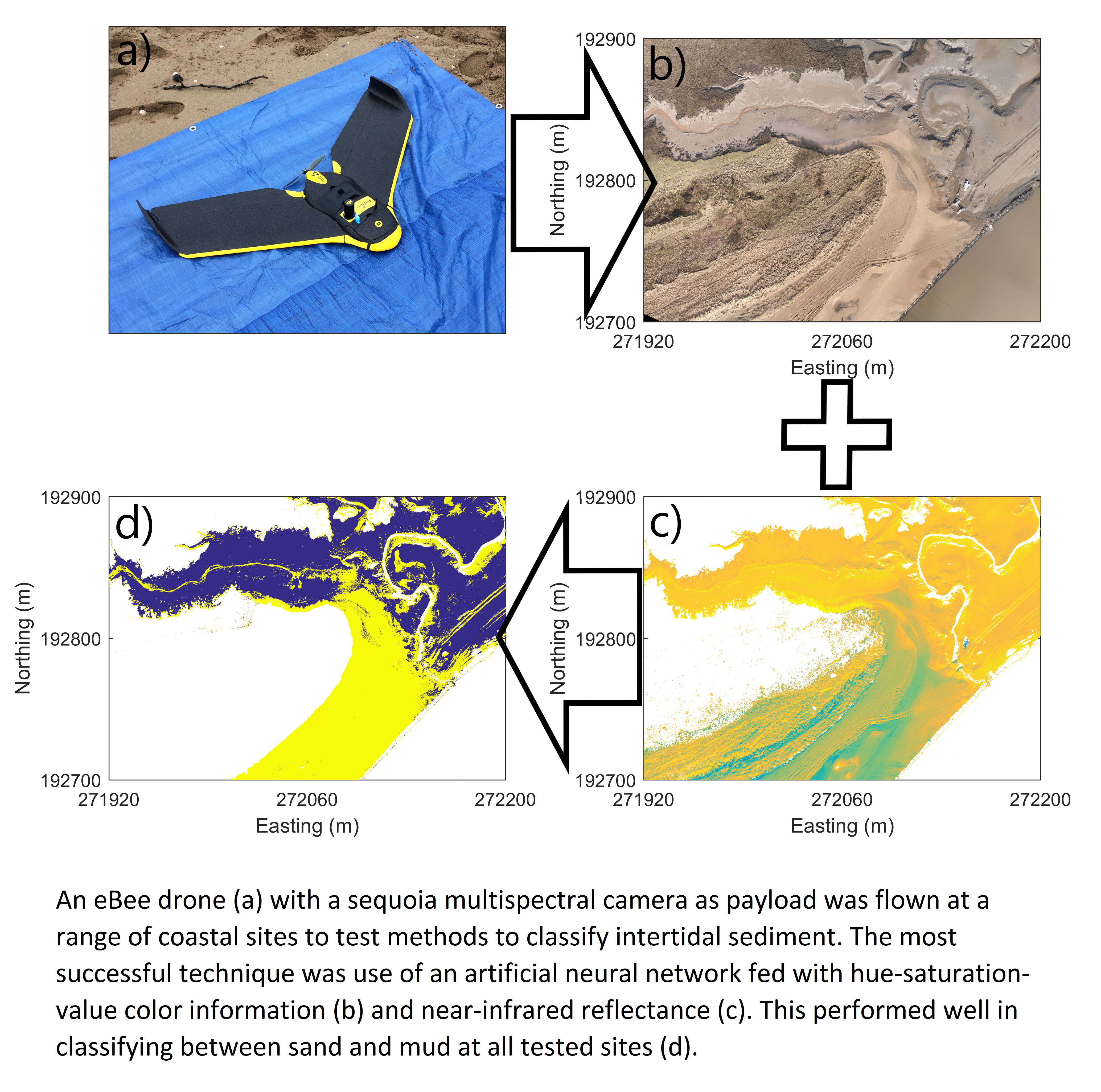
:This paper describes a new methodology to map intertidal sediment using a commercially available unmanned aerial system (UAS). A fixed-wing UAS was flown with both thermal and multispectral cameras over three study sites comprising of sandy and muddy areas. Thermal signatures of sediment type were not observable in the recorded data and therefore only the multispectral results were used in the sediment classification. The multispectral camera consisted of a Red–Green–Blue (RGB) camera and four multispectral sensors covering the green, red, red edge and near-infrared bands. Statistically significant correlations (>99%) were noted between the multispectral reflectance and both moisture content and median grain size. The best correlation against median grain size was found with the near-infrared band. Three classification methodologies were tested to split the intertidal area into sand and mud: k-means clustering, artificial neural networks, and the random forest approach. Classification methodologies were tested with nine input subsets of the available data channels, including transforming the RGB colorspace to the Hue–Saturation–Value (HSV) colorspace. The classification approach that gave the best performance, based on the j-index, was when an artificial neural network was utilized with near-infrared reflectance and HSV color as input data. Classification performance ranged from good to excellent, with values of Youden’s j-index ranging from 0.6 to 0.97 depending on flight date and site.

1. Introduction
A key aspect of both coastal research and environmental impact assessment for coastal development is the mapping of intertidal sediment type. This paper describes the use of a commercially available unmanned aerial system (UAS) to conduct such mapping. The focus of this work is on sands and muds. A key motivation for the work was the potential development of a tidal energy lagoon industry where altered intertidal coverage of sand and mud is perceived to be the primary environmental impact by both regulators and developers [1]. Gravels and cobbles are less important in this context: such sediment classes make up a much lower percentage of the intertidal in the areas of interest so are not considered a key receptor compared to sands and muds, which provide important benthic habitats. Additionally, the contrast between cobbles and sand is greater and hence they are considered less difficult to identify in remotely sensed data; the authors have previously demonstrated such distinction using terrestrial laser scanners [2].
Intertidal sediment type is important for two main reasons: benthic habitats and coastal morphodynamics. Grain size dictates the makeup of benthic communities (e.g., [3,4,5,6]); even temporally varying fine-scale sedimentological variations such as sedimentological differences between peaks and troughs of mega ripples can force differences in community structure [7]. Therefore, anthropogenically forced variations in grain size can affect community structure [8,9]. From a morphodynamic perspective, grain size and cohesive properties not only dictate thresholds of erosion and deposition [10,11]—beach profile is related to grain size, as well e.g., [12,13]. In an estuarine context, mud levels can influence long-term morphological development [14]. Episodic coastal mud events have been shown to have impacts on both hydrodynamics and morphodynamics, as well as having societal implications [15].
Alteration of wave exposure and tidal currents from the pre-existing baseline, whether due to coastal development, climate change or other factors, can lead to changes to baseline sediment coverage [16,17]. For example, an area of increased shelter may lead to increased deposition of muds or, vice versa, increased currents may erode finer sediment. To capture any changes, pre- and post-construction monitoring is desirable, particularly for large-scale developments. Seasonal variation in sediment supply or wave and tidal forcing mean that in some areas seasonal changes in sediment coverage may be observable (e.g., [18]) and hence regular monitoring may be required.
Direct sediment sampling and lab-based analysis is the default methodology for determining grain size and sediment type. For many estuarine areas and areas of high tidal range, the width of the intertidal expanse means that such in-situ monitoring is time consuming. This means mapping is based on a sparse grid of samples that may not accurately represent detailed 2-dimensional spatial patterns of different sediment types. Additionally, some intertidal areas are inaccessible by foot and there are health and safety considerations related to working in unconsolidated sediment and close to the low tide line.
Previously, researchers have demonstrated the use of satellite and aircraft remote sensing to map intertidal sediment with good success. Multispectral and hyperspectral instruments attached to light aircraft have been used to map clay content and intertidal grain size distributions [19]; to map percentages of sand, clay and silt and hence classify sediment type [20] or to classify intertidal areas into different classes [21,22,23]. Similarly, a range of satellites has multispectral or hyperspectral sensors that can be used to map intertidal sediment type [24,25] or estimate grain size [26]. These techniques have all been shown to perform well and facilitate classification of large areas of intertidal sediment in a time effective manner. However, the cost of instrumentation and deployment; the large quantities of data; and the specialist knowledge required for processing and interpretation mean they may not be suitable for routine environmental impact assessment work. In such cases, commercial consultancy companies may be more likely to use off-the-shelf tools to acquire data and UAS remote sensing may be more attractive.
In recent years, the use of UAS has proliferated in both academia and industry to facilitate a range of surveys. Typically, this focuses on the use of Red-Green-Blue (RGB) color images to reconstruct digital surface maps, (DSMs), through structure from motion (SfM) techniques. Industrial uptake means a range of off-the-shelf products are available including aircraft, sensors and pre- and post-processing software. One area that has embraced the use of UAS is precision agriculture, which means that relatively low-cost multispectral sensors are available. These are optimized for plant health monitoring and typically include spectral bands in the visible, red-edge (RE), and near-infrared (NIR), regions of the electromagnetic spectrum. Equally, thermal cameras are readily available for tasks such as inspection of solar panels. Past research has shown that thermal signals can be used to classify sediments: sandy sediments have a much stronger response to heating than muddy sediments [27]. The difference is caused by differences in sediment composition and porosity [28].
Here, both thermal and an agriculturally focused multispectral sensor were tested at three sites (Figure 1) on a small fixed wing UAS. Variation of the UAS measured parameters over the intertidal and their relationships with grain size and moisture content is presented. Next, different sets of the measured data channels were passed to three different classification routines. These routines were used to define different sediment type regions; a binary discrimination between ”sand” and ”mud” was considered. The three classification routines tested were: k-means clustering; artificial neural networks (ANNs) and the random forest (RF) approach.
The k-means technique was selected as it provides an example of an unsupervised technique which would allow efficient automation of the process and has previously been applied to sediment classification of intertidal areas [29]; ANNs were utilized because the authors have previously had success with ANN for sediment discrimination using terrestrial laser scanner data [2]; while the RF technique has been reported as a useful tool for classification of sediment type in remotely sensed data [30]. The objective of the study is to demonstrate the potential of low-cost, off-the-shelf UAS to map intertidal sediment type. The motivation is to facilitate the uptake of this new technology for both commercial and research applications.
2. Materials and Methods
The methodology is split between the study sites, field methodology and classification methodologies. Within the field methodology section is a description of the flight process, the lab-based sediment analysis and the initial post processing of the flight data. The classification methodology section describes the three techniques used and the metric used to compare them.
2.1. Field Methodology
2.1.1. Flight Methodology
Flights were conducted with both the senseFly ebee (Neath Estuary flights, see Section 2.1.3) and senseFly ebee Plus drones (additional sites). Flight details are given in Table 1. Both drones are fixed wing, powered by a single electric motor and propeller and are launched by hand. The Ebee is 0.7 kg in weight with a wingspan of 0.96 m whilst the Ebee Plus is 1.1 kg and has a wingspan of 1.1 m. In terms of nominal coverage, at 120 m the Ebee can cover 140 ha and the Ebee Plus 220 ha in one flight.
Two different sensors were used: a Parrot Sequoia multispectral sensor and a senseFly thermoMAP thermal camera (both purchased in the UK via Korec group). The Sequoia camera includes a rolling shutter RGB camera and four multispectral sensors covering the green (530–570 nm), red (640–680 nm), red edge (730–740 nm) and near-infrared (770–810 nm) bands. An upward facing sunshine sensor with the same four spectral bands allows for self-calibration of the reflectance values. Additional calibration was conducted prior to each flight using a reflective target.
The thermoMAP camera, which was only used at the three flights at the Neath Estuary, measured thermal infrared radiation in the range 7.5–13.5 µm which corresponds to a temperature range of −40 to 160 °C with a resolution of 0.1 °C.
Flights were planned using the senseFly eMotion 3 software. The surveyed area was kept the same for both sensors. Flight area was defined based on area of interest, consideration of obstructions, maximum flight time and the 500 m permitted working radius as specified by the UK Civil Aviation Authority. The size of the area of interest was reduced for the Neath site after the first flight. The flight software calculated the flight path based on specification of a required ground pixel resolution and expected wind speed. Ground pixel resolution varied between 6–9 cm for the multispectral sensors and was set at 10 cm for the thermal cameras. Both lateral and longitudinal overlap was set to 75% for all flights. Where both sensors were flown, the multispectral sensor was always flown first; the rationale being to ensure UAS measured temperature was as temporally close to point temperature measurements as possible. The same software was used for flight operation. Flights were fully automated and conducted on autopilot from take-off to landing. The thermoMAP camera was flown in time lapse mode (continual photo recording) whereas the Sequioa was flown in photo mode. All flights were conducted on the outgoing tide as close to low tide as possible (Table 1).
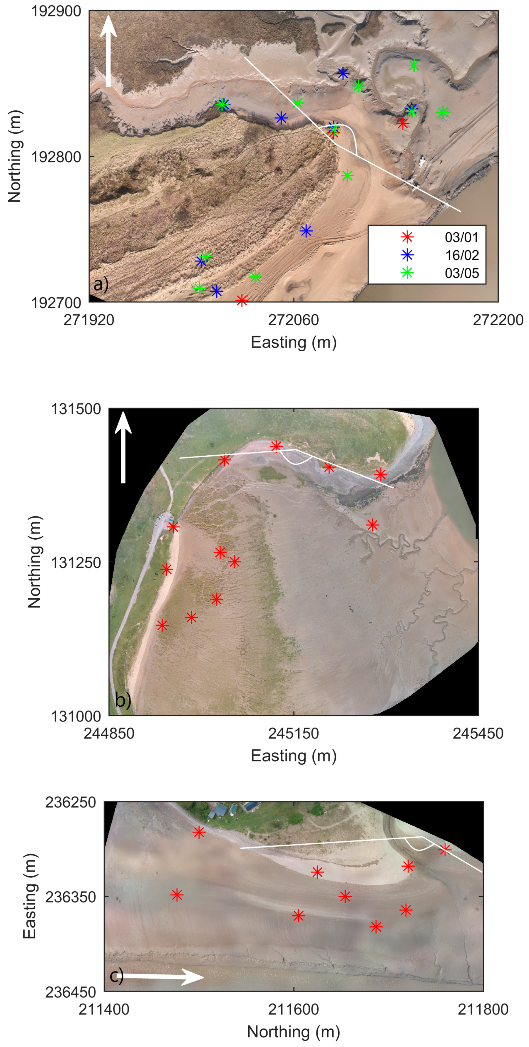
Prior to flying, ground control points (GCPs) were set out and their position surveyed using RTK-GPS to enable accurate geolocation. GCPs were created from black and white chequered lino that was cut into squares with two white and two black quadrants. Each quadrant had an edge length of 24 cm. To facilitate identification in the thermal imagery, the white sections were covered in aluminum foil, increasing the thermal contrast. It was aimed that GCPs would be evenly distributed about the study area (Figure 2); however accessibility of the intertidal limited this. Note that not all GCPs are shown for the first flight, which covered a wider area than subsequently analyzed. Number of GCPs per 100 photos ranged from 1.8 (Appledore) to 5.9 (Neath flight on 03/05/2018); this means that all flights have a reasonable number of GCPs [32].
2.1.2. Additional Measurements
To support analysis of the drone measured data, point measurements of sediment temperature and moisture content were taken. These were taken immediately after completion of both flights. The positions of points were measured with a Topcon HiPer HR RTK GPS. A Fisher Scientific Traceable flipstick thermometer with 0.1 °C resolution and 0.3 °C accuracy was used for the surface temperature measurements. A Delta-T ML3 ThetaKit was used to measure surface moisture. This device had an accuracy of ±1% and was chosen for its wide temperature and salinity operating ranges.
To test the classification performance, a classification of the sediment into ”sand” or ”mud” was made at specific points; this classification was made based on granularity and color of the surface sediment. For a sub sample of these, sediment samples were collected and processed to ground-truth the visual classification (see Section 2.1.3). Sediment surface samples were collected in the field using a stainless-steel combination auger to a 5-cm depth. In the laboratory, samples were oven-dried at 40 °C until dry before clays were disaggregated using a ceramic pestle and mortar. Sediments were passed through a 1-mm stainless sieve to remove stones, shells and larger pieces of organic matter and the sediment mass of the <1-mm grain-size fraction recorded. For particle-size determination analysis, the dry sediment samples were fully homogenized before sub-samples weighing 6 g were taken. These samples were chemically treated to remove organic matter. Particle size was determined in a Beckmann Coulter LS230 instrument that utilizes laser diffraction and measures particle sizes from 0.04 to 2000 µm in a wet module and to ISO 13320:2009 standards. All samples were analyzed using an automatic measurement mode using a Standard Operating Procedure (SOP), created prior to analysis. Samples were calibrated according to Thermo Scientific™ National Institute of Standards and Technology, (NIST), traceable size-standards of 15-µm, 50-µm and 200-µm nominal diameters. Values of median grain size were used to classify samples based on the Wentworth–Udden Scale. Results from the sediment analysis are presented in the study site description rather than results.
2.1.3. Study Sites
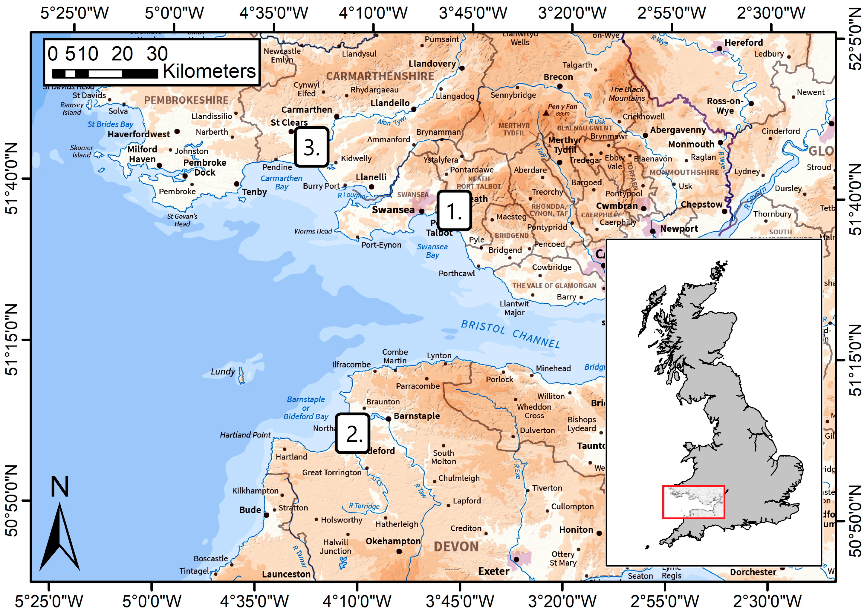
Three UK study sites were used in this investigation: the Neath Estuary (South Wales) flown three times to develop the optimum classification methodology and then two further sites flown to test the wider applicability of the methodology. These two additional sites were at Appledore (North Devon) and Llansteffan (South Wales). The site locations are shown in Figure 1. Orthomosaics of drone imagery for all three sites are displayed in Figure 2 and panoramic photos in Figure 3.
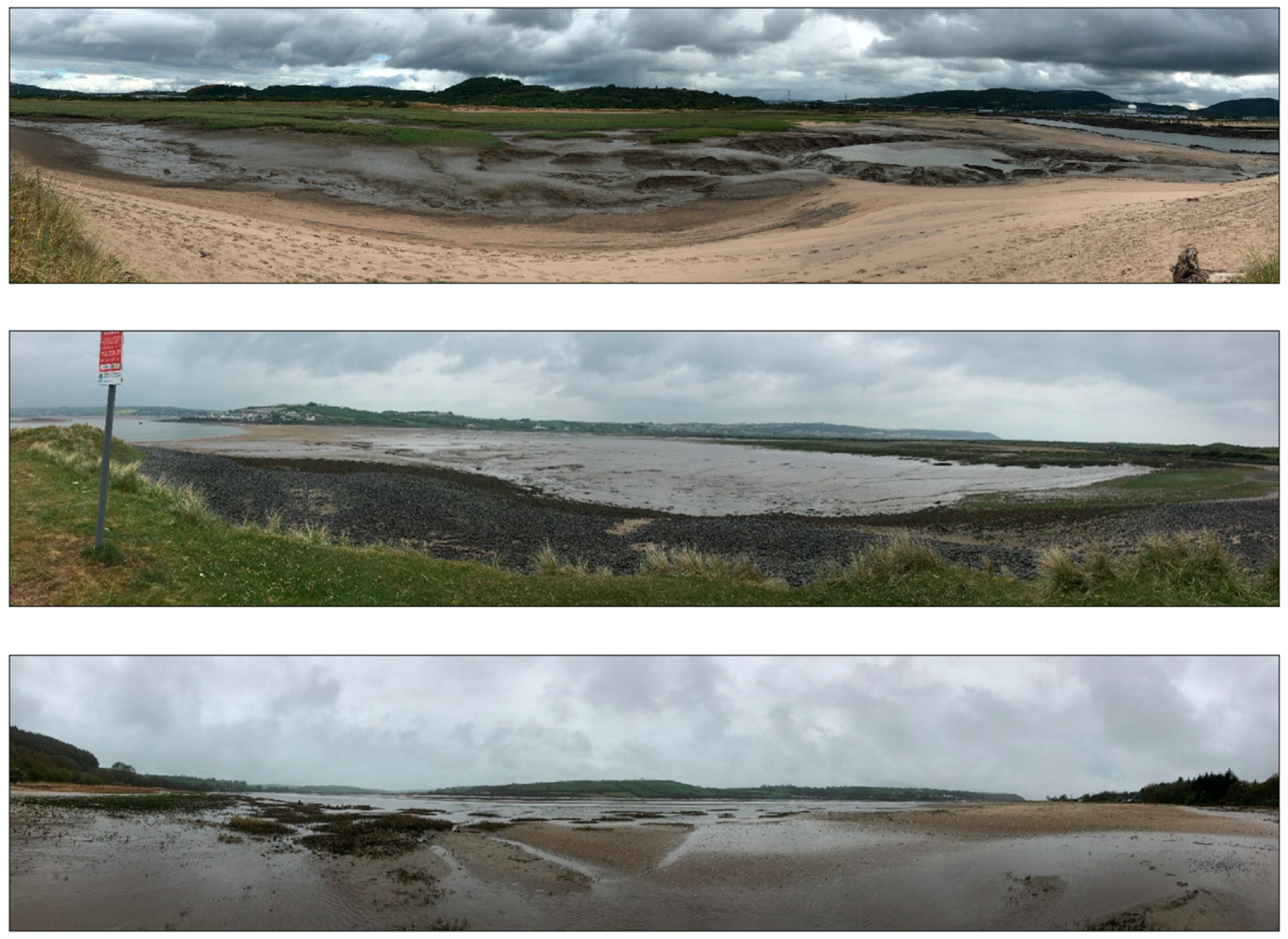
The Neath Estuary site is located where the Neath river meets the open sea. It is comprised of a central ridge of sand dunes with salt marsh and muddy creeks to the north and open sand beach to the south. The site is bounded to the east by the estuary. The topography of this site is highly three-dimensional caused by the presence of the Neath River and small creeks draining the muddy area in the lee of the sand dunes. Areas defined as ‘sand’ in the visual classification were medium sand with an average d50 of 294 µm; these areas had minimal mud content with less than 2% volume below 63 µm (the sand threshold on the Wentworth–Udden scale). Areas defined as “mud” had a d50 varying between 97 µm (very fine sand) and 158 µm (fine sand), however the percentage of mud increased to between 14–38%. During the time period of the test flights there was significant beach sediment recycling activities taking place just to the south of the study area. Visually this seems to increase the sand areas in the section to the north east of the small creek.
The second study location was at Appledore in North Devon at a site locally known as “The Skern”. This site was bounded by cobble and sand dunes to the north, west and south and by the estuary on the east. The site showed less three-dimensionality than the Neath Estuary site but there were still some drainage creeks present, particularly in the lower intertidal. The upper intertidal comprised of sand and well-established saltmarsh with muddy areas and pioneer saltmarsh in the middle intertidal. The lower intertidal was more spatially varying due to the presence of drainage creeks and varied between sand, mud, and muddy sand.
Visual samples defined as “sand” were fine sand on the Wentworth–Udden classification with d50 values between 185–227 µm. Points visually classified as ‘mud’ ranged from medium to coarse silt (31–39 µm).
The final site is at Llansteffan on the River Towy in South Wales. Whereas the other sites were at the seaward edge of estuaries, this site was further upstream and more two-dimensional. It consisted of a sandy upper intertidal and a muddier lower intertidal, with gradual gradation between the two across the intertidal profile. Correspondingly d50 reduced across the profile from 177 µm (fine sand) to 94 µm (very fine sand). Measured sediment samples that were visually classified as sand had less than 3% volume mud while the samples visually classified as mud had volumes between 16–39% of mud-sized particles.
2.1.4. Post-Processing of UAS Data
Prior to detailed analysis, the UAS collected data were post processed in four stages; firstly, flight logs and images were imported and georeferenced using the eMotion 3 software; secondly, the Pix4D software was used to generate color orthomosaics and index maps of multispectral reflectance; thirdly, GeoTIFF images created by Pix4D were resampled onto the same 0.1 m grid; finally, all data was screened to remove non-sediment areas.
The first stage is automated and requires minimal user intervention. The second stage of this process is more complex and includes initial processing; refinement of geo-location through marking of GCPs; followed by densification of the point cloud and generation of orthomosiacs and reflectance maps. The SfM approach used in Pix4D is described by [33]: the initial keypoint extraction and matching is based on binary descriptors [34]; a block bundle adjustment based on [35,36] is then conducted to determine internal and external camera parameters. Within the Pix4D software is a range of templates to optimize processing: for this study the ThermoMAP camera template was used for thermal imaging flights and the Ag Multispectral and Ag RGB templates used for imagery from the Sequioa. At this stage in the process, manual identification of the ground control points in the images was conducted using Pix4D’s ray cloud editor. Average root mean square error (RMSE) in GCP location varied between 0.026 m and 0.27 m, which was deemed acceptable for this work. Subsequently the point cloud is densified and then DSMs, orthomosaics, and reflectance maps created. In the third stage, the GeoTIFF images were interpolated onto one 0.1 m resolution grid covering the area of interest. At this point in the process careful visual inspection was conducted to asses that there were no odd features in the generated maps and that geolocation of all maps matched.
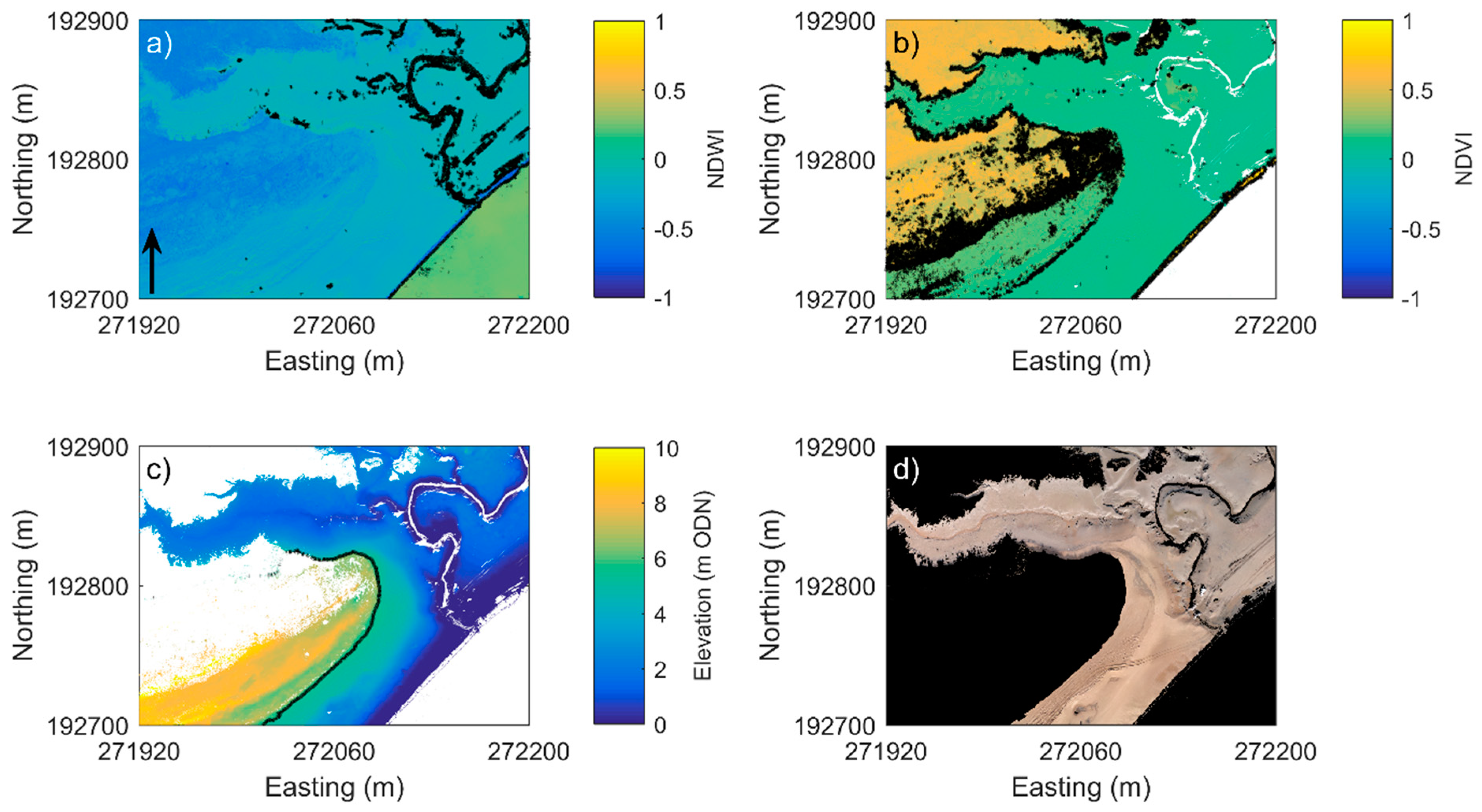
The fourth stage was the screening process, which removed open water, vegetation, and supratidal areas so that the areas left were predominantly bare intertidal sediment. Open water pixels were removed using the normalized difference water index (NDWI) [37]. This index is calculated as:
where Xgreen is the reflectance in the green band and XNIR is the reflectance in the near infra-red band. Positive values of this index are considered open water and thus are removed Vegetation was removed using the normalized difference vegetation index NDVI (Equation (2)):
Values over 0.3 were considered to be vegetation and removed following [38]. In Equation (2), Xred is the reflectance in the red band. A DSM created in Pix4d was used to remove supratidal areas based on the level of highest astronomical tide at the nearest national tide gauge network station. An example of this screening process is given in Figure 4.
2.2. Classification Methodology
One unsupervised and two supervised classification routines are tested here; unsupervised routines classify the data a priori based on characteristics of the dataset whereas supervised routines require some form of user input for training, typically definition of pre-classified subsets of the data. The unsupervised method used is k-means++ cluster-based classification [39] and the two supervised routines are based on artificial neural networks (ANNs) and on random forests [40]. All methods make use of built in MATLAB routines. Only data from the Sequioa sensor was fed to the classification routines, (see the reasoning in Section 3.1).
The RGB data was also transformed to the HSV colorspace: past research has suggested HSV may be better than RGB for image classification because there is less covariance in the HSV colorspace [41,42,43,44,45]. This gives 10 available data channels and the performance of 9 sets of these were considered. The 9 sets tested were: RGB; HSV; the multispectral channels (MS); RGB and MS; HSV and MS; RGB, red edge (RE) and near-infrared (NIR); HSV, RE and NIR; RGB and NIR; HSV and NIR. Required input for each technique was an n by m matrix where n is the number of samples and m is the number of data channels (between 3–7 dependent on set of data). Therefore, gridded data was transformed to vectors to conduct the analysis and then the output transformed to gridded classification maps.
The k-means algorithm [46] is a process that seeks to partition a set of n datapoints χ into k subsets, or clusters, based on minimizing the mean distance of points in a cluster to the centroid of that cluster. The k-means++ algorithm is a modification of the original k-means algorithm to improve the initial seeding process [39] by seeking starting centroids at data points that are relatively distant from existing centroids. Ref. [39] show that this approach both speeds up computational time and improves cluster definition. Since there is no supervision, the clusters of data are defined based purely on the data itself. It was found that while setting k to 2 did routinely split between sand and mud, data screening prior to classification was required (Section 2.1.4).
For the supervised classifications, subsets of the data where the sediment type was known was used to train the classification technique before the technique was applied to the whole area of interest. The first supervised classification technique tested was an ANN approach. A two-layer feed forward ANN was used [47]. The hidden layer has a sigmoid transfer function which enables a probability to be assigned to each classification. Sensitivity testing with different numbers of hidden neurons showed no statistically significant difference in classification performance and therefore the default value of 10 neurons were specified for the hidden layer. The number of neurons in the output layer is equal to the number of classes of sediment being discriminated between. The network was trained for weight and bias of the connections between neurons using the scaled conjugate gradient method [48]. Output is a k by n vector where k is the number of sediment classes and n is the number of data points, populated with probabilities that a specific point is a specific sediment class. Every data point was assigned the class that had the highest probability for each point.
The second supervised approach used was the random forests (RF) approach [40]. This approach uses a bootstrap aggregated ensemble of decision trees that avoids the likelihood of overfitting when using a single decision tree. Thirty trees were used in the forest: sensitivity testing with between 10–320 trees showed no statistical difference in classification performance.
To compare the different results, comparison was made between the visually classified field samples and points extracted from the classification maps. Confusion matrices were used which give clear insight into the performance of a classification technique; the structure is given in Table 2. Confusion matrices provide intuitive description of how well a methodology is performing; however, in order to rank the different methodologies, Youden’s index is used [49]. This is calculated as:
where j is Youden’s index and the other quantities are as Table 1. The j-index has values ranging from −1 to 1 with 1 indicating a perfect classification.
3. Results
3.1. Variation of Measured Parameters over the Intertidal
Temperature and moisture were measured at a range of locations for the three flights at the Neath Estuary sites. Figure 5 shows the variation of these parameters. The left-hand panel shows a comparison of UAS measured temperature against point measured temperature; it demonstrates that the two are strongly related (r = 0.96; significant at 99% level) and that UAS-derived temperatures reliably reproduce intertidal temperature in this case. The central panel shows a comparison between point-measured moisture content and point-measured temperature: for the first flight there is a positive correlation (r = 0.59), significant at the 95% level; there is no correlation for the second flight; for the third flight there is a strong negative correlation (r = −0.82) also significant at the 95% level.
This indicates the variability in the influence of moisture content on temperature with other environmental parameters. There is negligible clustering of the different sediment types. The right-hand panel shows variation of point-measured moisture content with point-measured elevation: for all flights there is a negative correlation that is statistically significant at the 95% level. This is unsurprising since points lower on the profile will have had less time to dewater as the tide recedes. While all points with lower moisture contents are sand, there are no mud points higher up the intertidal profile and lower on the profile sand and mud have similar moisture contents.
To further explore temperature variation, Figure 6 shows maps of temperature for the three flights. For all panels, color shading indicates UAS-measured temperature and black contours the morphology. The upper panel shows the first flight (30/01/2018), due to low temperatures, there was insufficient thermal contrast to enable orthorectification of the entire area of interest. There is a sharp break in temperature in the sand portion of the study area; further consideration showed this. matched the level of the previous high tide (red line in image). The second and third flights both had sufficient thermal contrast to enable the entire area to be orthorectified. For the second flight (16/02/2018) the temperature variation seemed related to angle of slope of the morphology, with northward facing slopes being cooler than southward facing slopes (angled towards the sun). The third flight (03/05/2018), when temperatures were higher and when the sun was more directly overhead showed more uniform variation. Temperatures were lower at lower elevations. As shown in Figure 5 there is a strong negative correlation with moisture content. No clear links between temperature and sediment type were observed for any of the flights. Therefore, results from the thermal camera were not included in the classification analysis and it is believed that thermal cameras are unsuitable for year-round monitoring of sediment type in a Northern European context.
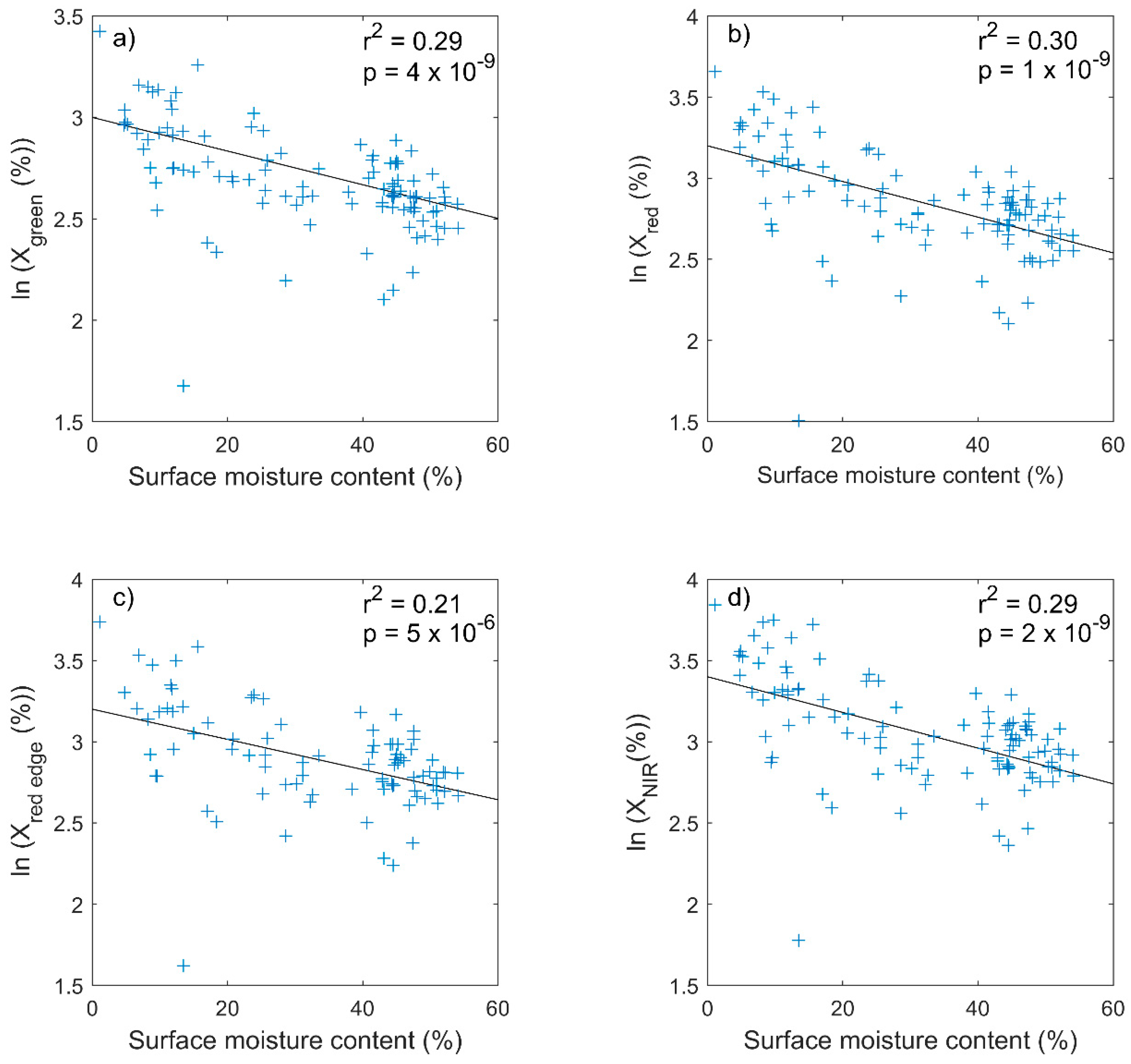
Consideration was given to the comparison between multispectral reflectance and both moisture content (Figure 7) and measured grain size (Figure 8); where the reflectance is presented as a percentage (the reflected intensity divided by the incident intensity multiplied by 100). Based on Beer’s law, that grain size and moisture content are exponentially related to intensity [50], the natural log of reflectance is plotted against the tested properties. Faulty calibration meant the red edge reflectance was incorrectly scaled for the flight on 30/01. Therefore, it is ignored for this part of the analysis; since the error was a scaling factor but the shape of variation was correct, it was still utilized in the classification testing (see Section 3.2). Surface moisture content was only available from the three Neath flights; data from all flights is combined in Figure 7. There is a negative correlation for all spectral bands; while r2 values are low (values marked on figure), p values indicate that the correlation is highly significant (>99% level).
The comparison between median grain size and natural log of the spectral reflectance is shown in Figure 8. Data from all flights and sites are combined in this plot. For all multispectral channels, there is a positive trend to the relationship. Correlations are significant at the 99% level for the green, red and NIR channels (values marked on Figure 8); while the red edge correlation is only significant at the 95% level. Similar to the comparison against surface moisture content; while statistically significant, r2 values are low which indicates the range of parameters affecting reflectance. The statistically significant correlation between grain size and NIR reflectance raises the question as to whether UAS measured reflectance could be used to directly map grain size.
A linear best fit to the data in Figure 8d gave the equation:
where XNIR(%) is the percentage NIR reflectance.
This was used to estimate grain size and estimated values are plotted against measured grain size in Figure 9. The equation of the line of best fit is displayed on this figure; it approaches a 1:1 fit suggesting there is potential in the approach. However, there is a large amount of scatter in the data, as indicated by the r2 value of 0.38. Therefore, this approach is taken no further in this paper; although some comment is made in the discussion (Section 4).
3.2. Classification Results
3.2.1. Neath Estuary Classification
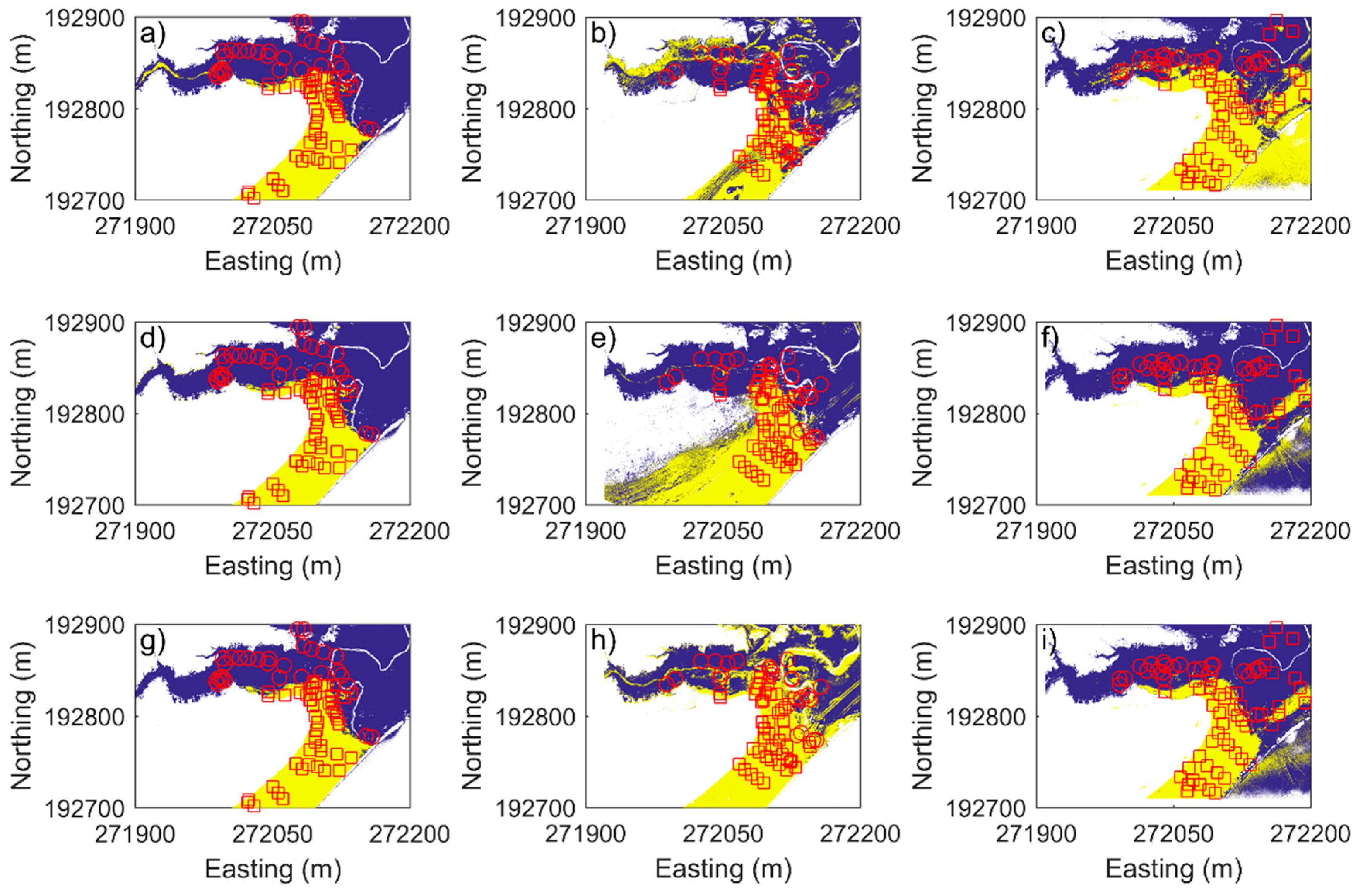
The classification routines and sets of input data were tested and ranked based on Youden’s index (Section 2.2). While reference is made to mud, dependent on site, this may refer to muddy sand (see Section 2.1.3). The best two sets of data and their j values for each flight and classification routine is shown in Table 3 and classification maps for the optimum set of data for each routine in Figure 10. In general, classification is performing well with optimum j values between 0.65 and 0.99. Table 3 shows that there is a range of sets of data channels giving the optimum results. Apart from the random forest classification on the 30/01/2018 (which had joint optimum between HSV alone and HSV + NIR), the optimum classification makes use of some or all of the multispectral sensors.
Statistically, based on standard error [36], there is no difference in performance between the different flights, classification methodologies or rank for the optimum methodologies (Table 4). Considering the average j values for each classification shows that in general the best performing is the artificial neural networks (average j = 0.88); the average j value for the k-means classification was 0.84 and the average value for the random forest classification was 0.82. Figure 10 presents classification maps for the optimum set of data channels for each methodology and flight. For flight one (30/01), all spatial maps are similar which is reflected in the very similar j values. There are obvious errors in both the k-means and RF classifications for the second flight with areas of mud around the creek flanks classified as sand. The ANN approach appears to perform much better for this flight. For the third flight, again all classification techniques give very similar classification maps. This is unsurprising since all optimum sets have the same j value (0.81).
Given the statistical similarity between the different classification schemes and sets of input data (Table 4); a point-based ranking was used to establish which set of input data was most likely to give the best results. Using the data in Table 3, from all flights and classifications, 2 points were assigned every time a set of input data was the optimum classification and 1 point when the set of input data was the second-best performing classification. These points were then summed for the 9 sets of input data and the results are shown in Table 5. By far the highest-ranking set is the combination of HSV and the NIR channel. This is perhaps unsurprising as the NIR channel had the best correlation with grain size (Figure 8). Based on this information, and the fact that on average ANN classification performed best, the optimum methodology was defined as an ANN classification using HSV and NIR as input data.
Confusion matrices for this approach for the three Neath flights are shown in Table 6, Table 7 and Table 8 and classifications are visually represented in Figure 11. For flight one, all the mud points were correctly predicted as mud and only two sand points were falsely classified as mud; this gave a value for j = 0.97 which indicates an excellent classification. There was greater misclassification for the second flight giving a value of j = 0.6, but the classification can still be considered reasonable. Of the 23 mud points 8 were misclassified as sand and one of the 48 sand points was misclassified as mud. The areas of mud classified as sand can be seen in Figure 11e. The third flight once again provided a good classification with a value of j = 0.81. All mud points were correctly classified and of the 48 sand points, 39 were correctly classified.
3.2.2. Tests at Alternative Sites
The methodology provided good results at both additional sites (j = 0.64 at Appledore and j = 0.71 at Llansteffan). Confusion matrices are shown in Table 9 and Table 10 and visual representation in Figure 12 and Figure 13. At Appledore these is a similar amount of misclassification for both class of sediment. Areas where mud has dried out are sometimes classified as sand and some wet sand point classified as mud. At Llansteffan all areas defined as mud were correctly classified, but some sand areas were classified as mud. Fast moving variable cloud cover was present at the time of this flight which is evident in the orthomosaic and may help explain some misclassification.
4. Discussion
This paper has demonstrated the ability to distinguish between sandy and muddy intertidal sediments using a UAS with RGB and multispectral sensors. In this analysis, the optimal classification made use of HSV color and NIR reflectance data. Other research [33,34,35,36,37] has demonstrated that HSV is better than RGB for image classification and these results corroborate those findings. The benefits of including NIR reflectance is unsurprising since a positive correlation between median grain size and NIR reflectance was found.
The positive correlation between grain size and multispectral reflectance has been noted by other researchers using satellite remote sensing [26] and this relationship has been used to map grain size. Future work will conduct more flights and analyze more point sediment samples to widen the grain size parameter space and endeavor to develop similar tools for use with UAS sensors.
Despite the statistically significant positive correlation between multispectral reflectance and values of d50, there was a large amount of scatter in the data. A more statistically likely relationship was noted between multispectral reflectance and surface moisture content. Surface moisture and grain size are related because areas of coarser sediment will typically dewater faster and hence have lower surface moisture values than areas of finer sediment. Over the intertidal area, this is complicated by variation in dewatering affected by elevation and tidal inundation, as well as spatially varying groundwater influences. It is possible that by including elevation maps and time of flight from previous high tide, some correction could be made for this complicating factor. Future work is planned to address this aspect.
Very similar results were found for all sets of data and classification routines. This is partially due to the data screening prior to classification where both vegetation and open water were removed. The motivation for applying this screening process was that without the screening the unsupervised k-means routine failed to split between sediment types, instead regularly creating one class that was predominantly vegetation and one class predominantly bare sediment. Increasing number of classes did not improve classifications. Therefore, it was deemed a fairer test if only bare sediment was passed to the classification routines. Constraining the classification problem in this way was fast, automatable and transparent (relying on well know indices); therefore, it is not seen as a limitation of the study. Should classification of these regions be of interest, a multi-stage classification could be used to classify (rather than remove) regions of vegetation and water using the method described prior to the sediment classification.
The technique could easily be applied to other broad scale classes such as bedrock and gravel and vegetated intertidal areas can be identified using the NDVI. Future work will consider splitting into more detailed sediment classes. Results from the Neath Estuary where the “mud” portion was actually a mud–sand mixture suggest that there are sufficient differences in UAS measured parameters that this should be feasible. Initial tests suggested that an unsupervised classification of greater than two sediment types did not work well. Therefore, it is likely that performance of classification into multiple classes will depend on ease of defining suitable training datasets.
The multispectral and RGB sensor used, the Sequoia, has a global shutter for the four multispectral sensors but a rolling shutter for the RGB sensor. A rolling shutter leads to inaccuracies in the images when used on a moving platform such as a drone because the sensor will move in between lines of pixels being exposed by the shutter. While the processing software, Pix4D, has a correction algorithm for rolling shutter cameras and errors are minimized by use of GCPs, some errors will remain. In this study, careful comparison of RGB, multispectral and thermal orthomosaics were undertaken to ensure accurate coreferencing away from GCPs and no obvious errors were noted. Therefore, it is believed that the orthomosaics are suitable accurate for the purposes of the study. The DSMs are less likely to be accurate and the product literature cautions against relying on DSMs from the rolling shutter RGB. In this study elevation is only used to screen the supratidal area and little error in this application was noted. Other similar sensors, such as the MicaSense RedEdge-M, are available with global shutter RGB cameras, which would remove this uncertainty. Alternatively, a subsequent flight with a global shutter RGB camera would provide more accurate color information.
Remote sensing of intertidal sediment has several benefits over ground-based sampling, typically undertaken on foot. Most importantly, from a logistical perspective, is the reduction in health and safety risk associated with working in unconsolidated sediment close to the low tide line; additionally, time in the field can be significantly reduced which may reduce survey cost. Spatial resolution is much higher which avoids errors in classification caused by interpolation between a sparse network of samples.
Deployment of UAS fit well within the context of other remote sensing options such as airborne or satellite remote sensing. The technique is much lower cost than methods using manned aircraft which facilitates multiple repeat surveys, as required to capture seasonal change or the rapid adjustment to new coastal developments. The higher pixel resolution, compared to both satellite and manned aircraft solutions, mean smaller scale change could be identified. Additionally, the commercial availability of monitoring solutions is attractive and would make uptake by researchers, industry, governmental and nongovernmental agencies easier. However, the set-up of commercially available sensors is relatively inflexible. Past research has shown that reflectance in the short and medium wave infrared bands is more useful for sediment classification, and that hyperspectral sensors can accurately map geological properties of rock, e.g., [51]. Recent studies have mounted hyperspectral cameras to drones for a range of purposes [52,53]. Such approaches would likely provide better results; however, the sensors are expensive [52] and flight duration of drones suitable to mount the cameras is low [52,53], reducing extent of coverage.
Previous studies identified thermal infrared camera as having good potential for identifying regions of sand and mud [28]. Thermal cameras did not perform well in this study, however, which highlights the importance of other environmental factors in such discrimination. Areas where there is greater or more uniform solar heating may well show better success.
All UAS use is constrained by technical and regulatory factors. UAS regulations are defined by national aviation authorities. In the UK, regulations mean UAS must be flown within visual line of sight which limits distance of the UAS to 500 m from the operator; this distance can be extended by application for additional permissions, but they are not always granted. Another key regulatory factor is the 150 m separation distance from ”congested areas” which include any area regularly used for commercial, industrial or recreational purposes. Technical factors include takeoff and landing requirements and weather limitations. Fixed wing UAS such as used in this study can cover larger areas than an octocopter-type UAS, but require suitable landing areas such flat grass. In this study, sand areas of the beach were typically used, however this did constrain choice of suitable test sites. Octocopters can take off and land vertically and hence landing areas are not a restriction on site selection. In addition, weather conditions including wind speed, visibility and heavy rain must be considered. An analysis of 10 years of weather data from a station at Mumbles close to the Neath Estuary site showed that conditions were only suitable for flying 40% of the time.
5. Conclusions
This contribution explores the use of UASs to map intertidal sediment type. Flights were conducted with both a thermal infrared camera and a multispectral camera that measured red, green, red edge and near-infrared reflectance as well as RGB color. Use of the thermal camera for sediment mapping was discounted in a northern European context because preliminary study showed that other environmental factors controlled the temperature variation over the intertidal rather than sediment type. Relationships between both color and multispectral reflectance against surface moisture were identified. Importantly, there was also a positive correlation between median grain size and multispectral reflectance, with the best correlation using the near-infrared reflectance (r = 0.6, 99% significance).
Three classification routines (k-means, artificial neural networks and random forests) were tested with nine sets of UAS measured data to broadly discriminate between sand and mud in the intertidal. Prior to classification, the orthomosaics were screened for vegetation and open water, which constrained the problem. Inclusion of multispectral channels improved results over classifications just using color data. The optimum combination was an artificial neural network approach using HSV color and NIR reflectance, where over the 5 flights Youden’s j-index varied between 0.6 and 0.97, (where j = 1 corresponds to perfect classification). This approach was deemed very successful and it shows that UASs are a suitable tool for remote sensing of intertidal sediment.
Author Contributions
Conceptualization, I.F.; Formal analysis, I.F. and A.M.; Funding acquisition, I.F., M.T. and D.E.R.; Investigation, I.F. and A.M.; Methodology, I.F., A.M. and D.E.R.; Project administration, D.E.R.; Resources, M.T.; Supervision, D.E.R.; Writing—original draft, I.F.; Writing—review & editing, I.F., A.M., M.T. and D.E.R.
Funding
This work was conducted as part of the UK NERC funded DST-UAV project (NE/R014485/1). The authors acknowledge the financial support of the Welsh Assembly Government and Higher Education Funding Council for Wales through the Sêr Cymru National Research Network for Low Carbon, Energy and Environment.
Acknowledgments
Participation of project partners Natural Resources Wales, Natural England, AG surveys and Tidal Lagoon Power is acknowledged. The assistance of Richard Gauchwin from Korec Group with loan of the multispectral camera is also acknowledged. Datasets resulting from this work are available open access at DOI: 10.5281/zenodo.1626385.
Conflicts of Interest
The authors declare no conflicts of interest.
References
- Mackinnon, K.; Smith, H.C.M.; Moore, F.; van der Weijde, A.H.; Lazakis, I. Environmental interactions of tidal lagoons: A comparison of industry perspectives. Renew. Energy 2018, 119, 309–319. [Google Scholar] [CrossRef] [Green Version]
- Fairley, I.; Thomas, T.; Phillips, M.; Reeve, D. Terrestrial laser scanner techniques for enhancement in understanding of coastal environments. In Seafloor Mapping along Continental Shelves: Research and Techniques for Visualizing Benthic Environments; Finkl, C.W., Ed.; Springer International: New York, NY, USA, 2016; pp. 273–289. [Google Scholar]
- Anderson, M.J.; Ford, R.B.; Feary, D.A.; Honeywill, C. Quantitative measures of sedimentation in an estuarine system and its relationship with intertidal soft-sediment infauna. Mar. Ecol. Prog. Ser. 2004, 272, 33–48. [Google Scholar] [CrossRef] [Green Version]
- Rodil, I.F.; Lastra, M. Environmental factors affecting benthic macrofauna along a gradient of intermediate sandy beaches in northern Spain. Estaur. Coast. Shelf Sci. 2004, 61, 37–44. [Google Scholar] [CrossRef]
- McLachlan, A. Physical factors in benthic ecology: Effects of changing sand particle size on beach fauna. Mar. Ecol. Prog. Ser. 1996, 131, 205–217. [Google Scholar] [CrossRef]
- Rodrigues, A.M.; Meireles, S.; Pereira, T.; Gama, A.; Quintino, V. Spatial patterns of benthic macroinvertebrates in intertidal areas of a Southern european estuary: The Tagus, Portugal. Hydrobiologia 2006, 555, 99–113. [Google Scholar] [CrossRef]
- Van der Wal, D.; Ysebaert, T.; Herman, P.M.J. Response of intertidal benthic macrofauna to migrating megaripples and hydrodynamics. Mar. Ecol. Prog. Ser. 2017, 585, 17–30. [Google Scholar] [CrossRef]
- Manning, L.M.; Peterson, C.H.; Bishop, M.J. Dominant macrobenthic populations experience sustained impacts from annual disposal of fine sediments on sandy beaches. Mar. Ecol. Prog. Ser. 2014, 508, 1–15. [Google Scholar] [CrossRef] [Green Version]
- Vanden Eede, S.; Van Tomme, J.; De Busschere, C.; Vandegehucte, M.L.; Sabbe, K.; Stienen, E.W.M.; Degraer, S.; Vincx, M.; Bonte, D. Assessing the impact of beach nourishment on the intertidal food web through the development of a mechanistic-envelope model. J. Appl. Ecol. 2014, 51, 1304–1313. [Google Scholar] [CrossRef] [Green Version]
- Le Hir, P.; Cayocca, F.; Waeles, B. Dynamics of sand and mud mixtures: A multiprocess-based modelling strategy. Cont. Shelf Res. 2011, 31, 135S–149S. [Google Scholar] [CrossRef]
- Wu, W.; Perera, C.; Smith, J.; Sanchez, A. Critical shear stress for erosion of sand and mud mixtures. J. Hydraul. Res. 2018, 56, 96–110. [Google Scholar] [CrossRef]
- Benedet, L.; Finkl, C.W.; Cambell, T.; Klein, A. Predicting the effect of beach nourishment and cross-shore sediment variation on beach morphodynamic assessment. Coast. Eng. 2004, 51, 839–861. [Google Scholar] [CrossRef]
- Medina, R.; Losada, M.A.; Losada, I.J.; Vidal, C. Temporal and spatial relationship between sediment grain size and beach profile. Mar. Geol. 1994, 118, 195–206. [Google Scholar] [CrossRef]
- Braat, L.; van Kessel, T.; Leuvan, J.R.F.W.; Kleinhans, M.G. Effects of mud supply on large-scale estuary morphology and development over centuries to millennia. Earth Surf. Dyn. 2017, 5, 617–652. [Google Scholar] [CrossRef] [Green Version]
- Calliari, L.J.; Holland, T.; Pereira, P.S.; Guedes, R.M.C. The Influence of Mud on the Inner Shelf, Shoreface, Beach, and Surf Zone Morphodynamics; Cassino, Southern Brazil. In Proceedings of the Coastal Sediments’07, New Orleans, LA, USA, 13–17 May 2007. [Google Scholar]
- Ahn, I.-Y.; Choi, J.-W. Macrobenthic communities inpacted by anthropogenic activities in an intertidal sand falt on te west coast (Yellow Sea) of Korea. Mar. Pollut. Bull. 1998, 36, 808–817. [Google Scholar] [CrossRef]
- Wartel, S.; Chen, M.; van Eck, G.T.M.; van Maldegem, D. Influence of harbour construction on mud accumulation in the Scheldt estuary. Aquat. Ecosyst. Health Manag. 2007, 10, 107–115. [Google Scholar] [CrossRef]
- Lesourd, S.; Lesueur, P.; Brun-Cottan, J.C.; Garnaud, S.; Poupinet, N. Seasonal variations in the characteristics of superficial sediments in a macrotidal estuary. Estaur. Coast. Shelf Sci. 2003, 58, 3–16. [Google Scholar] [CrossRef]
- Rainey, M.P.; Tyler, A.N.; Gilvear, D.J.; Bryant, R.G.; McDonald, P. Mapping intertidal estuarine sediment grain size distributions through airborne remote sensing. Remote. Sens. Environ. 2003, 86, 480–490. [Google Scholar] [CrossRef]
- Castillo, E.; Pereda, R.; Luis, J.M.; Medina, R.; Viguri, J. Sediment grain size estimation using airborne remote sensing, field sampling, and robust statistic. Environ. Monit. Assess. 2011, 181, 431–444. [Google Scholar] [CrossRef] [PubMed]
- Thomson, A.G.; Fuller, R.M.; Yates, M.G.; Brown, S.L.; Cox, R.; Wadsworth, R.A. The use of airborne remote sensing for extensive mapping of intertidal sediments and saltmarshes in eastern England. Int. J. Remote Sens. 2003, 24, 2717–2737. [Google Scholar] [CrossRef]
- Deronde, B.; Houthuys, R.; Debrun, W.; Fransaer, D.; van Lanker, V.; Henriet, J.P. Use of Airborne Hyperspectral Data and Laserscan Data to Study Beach Morphodynamics along the Belgian Coast. J. Coast. Res. 2006, 22, 1108–1117. [Google Scholar] [CrossRef]
- Adam, S.; De Backer, A.; Degaer, S.; Monbaliu, J.; Toorman, E.A.; Vincx, M. Sediment characterization of intertidal mudflats using remote sensing. Proc. Mar. Sci. 2008, 9, 109–124. [Google Scholar]
- Yates, M.G.; Jones, A.R.; McGrorty, S.; Goss-Custard, J.D. The Use of Satellite Imagery to Determine the Distribution of Intertidal Surface Sediments of the Wash, England. Estaur. Coast. Shelf Sci. 1993, 36, 333–344. [Google Scholar] [CrossRef]
- Jung, R.; Adolph, W.; Ehlers, M.; Farke, H. A multi-sensor approach for detecting the different land covers of tidal flats in the German Wadden Sea—A case study at Norderney. Remote Sens. Environ. 2015, 170, 188–202. [Google Scholar] [CrossRef]
- Van der Wal, D.; Herman, P.M.J. Quantifying the particle size of intertidal sediments with satellite remote sensing in the visible light, thermal infrared and microwave spectral domain. In Proceedings of the ISPRS Commission VII Symposium ‘Remote Sensing: From Pixels to Processes’; Kerle, N., Skidmore, A., Eds.; ISPRS: Enschede, The Netherlands, 2006. [Google Scholar]
- Chickadel, C.; Thomson, J. Exploitation of Thermal Signals in Tidal Flat Environments (Award no: N00014-08-10809)—Final Report; Applied Physics Lab, University of Washington: Seattle, WA, USA, 2010. [Google Scholar]
- Thomson, J.; Chickadel, C.; Rinehimer, J.P. Classification of Intertidal Sediments Using Infrared Sensing. In Proceedings of the GO35C-08 AGU Ocean Sciences, Portland, OR, USA, 2–26 February 2010. [Google Scholar]
- Ibrahim, E.; Adam, S.; Monbaliu, J. Assesemnt of unsupervised classification techniwues for intertidal sediments. In Remote Sensing for a Changing Europe; Maktav, D., Ed.; IOS Press: Amsterdam, The Netherlands, 2009. [Google Scholar]
- Wang, W.; Yang, X.; Liu, G.; Zhou, H.; Ma, W.; Yu, Y.; Li, Z. Random forest classification of sediments on exposed intertidal flats using ALOS-2 quad-polarimetric SAR data. Int. Arch. Photogramm. Remote Sens. Spat. Inf. Sci. 2016. [Google Scholar] [CrossRef]
- Easytide Website. Available online: http://www.ukho.gov.uk/easytide/EasyTide/index.aspx (accessed on 3 May 2018).
- Sanz-Ablanedo, E.; Chandler, J.H.; Rodríguez-Pérez, J.R.; Ordóñez, C. Accuracy of Unmanned Aerial Vehicle (UAV) and SfM Photogrammetry Survey as a Function of the Number and Location of Ground Control Points Used. Remote Sens. 2018, 10, 1606. [Google Scholar] [CrossRef]
- Kung, O.; Strecha, C.; Beyeler, A.; Zufferey, J.-C.; Floreano, D.; Fua, P.; Gervaix, F. The accuracy of automatic photogrammetric techniques on ultra-light UAV imagery. In Proceedings of the UAV-g 2011—Unmanned Aerial Vehicle in Geomatics, Zürich, Switzerland, 14–16 September 2011. [Google Scholar]
- Strecha, C.; Bronstein, A.; Bronstein, M.; Fua, P. LDA-Hash: Improved matching with smaller descriptors. IEEE Trans. Pattern Anal. Mach. Intell. 2012, 34, 66–78. [Google Scholar] [CrossRef] [PubMed]
- Triggs, B.; McLauchlan, P.; Hartley, R.; Fitzgibbon, A. Bundle Adjustment—A Modern Synthesis. In Vision Algorithms: Theory and Practice; Triggs, B., Zisserman, A., Szeliski, R., Eds.; Springer International: New York, NY, USA, 2000; pp. 298–372. [Google Scholar]
- Hartley, R.; Zisserman, A. Multiple View Geometry in Computer Vision; Cambridge University Press: Cambridge, UK, 2004; p. 674. [Google Scholar]
- McFeeters, S.K. The use of the normalized difference water index (NDWI) in the delineation of open water features. Int. J. Remote Sens. 1996, 17, 1425–1432. [Google Scholar] [CrossRef]
- Yu, L.; Porwal, A.; Holden, E.-J.; Dentith, M.C. Suppression of vegetation in multispectral remote sensing images. Int. J. Remote Sens. 2011, 32, 7343–7357. [Google Scholar] [CrossRef]
- Arthur, D.; Vassilvitskii, S.; Siam, A. k-means plus plus: The Advantages of Careful Seeding. In Proceedings of the 18th Annual Symposium on Discrete Algorithms, New Orleans, LA, USA, 7–9 January 2007; pp. 1027–1035. [Google Scholar]
- Breiman, L. Random forests. Mach. Learn. 2001, 45, 5–32. [Google Scholar] [CrossRef]
- Ilea, D.E.; Whelan, P.F. Image segmentation based on the integration of colour-texture descriptors—A review. Pattern Recognit. 2011, 44, 2479–2501. [Google Scholar] [CrossRef]
- Kumar, G.; Sarthi, P.; Ranjan, P.; Rajesh, R. Performance of k-means based Satellite Image Clustering in RGB and HSV Color Space. In Proceedings of the 5th International Conference on Recent Trends in Information Technology, Chennai, India, 8–9 April 2016. [Google Scholar]
- Kusetogullari, H.; Yavariabdi, A. Unsupervised Change Detection in Landsat Images with Atmospheric Artifacts: A Fuzzy Multiobjective Approach. Math. Probl. Eng. 2018. [Google Scholar] [CrossRef]
- Su, L.H.; Gibeaut, J. Using UAS Hyperspatial RGB Imagery for Identifying Beach Zones along the South Texas Coast. Remote Sens. 2017, 9, 159. [Google Scholar] [CrossRef]
- Zhang, H.; Fritts, J.E.; Goldman, S.A. Image segmentation evaluation: A survey of unsupervised methods. Comput. Vis. Image Underst. 2008, 110, 260–280. [Google Scholar] [CrossRef] [Green Version]
- Lloyd, S.P. Least-squares quantisation in PCM. IEEE Trans. Inf. Theory 1982, 22, 129–137. [Google Scholar] [CrossRef]
- Svozil, D.; Kvasnicka, V.; Pospichal, J.Í. Introduction to multi-layer feed-forward neural networks. Chemom. Intell. Lab. Syst. 1997, 39, 43–62. [Google Scholar] [CrossRef]
- Moller, M.F. A scaled conjugate-gradient algorithm for fast supervised learning. Neural Netw. 1993, 6, 525–533. [Google Scholar] [CrossRef]
- Youden, W.J. Index for rating diagnostic tests. Cancer 1950, 3, 32–35. [Google Scholar] [CrossRef] [Green Version]
- Clark, R.N. Chapter 1: Spectroscopy of Rocks and Minerals, and Principles of Spectroscopy. In Manual of Remote Sensing, Volume 3, Remote Sensing for the Earth Sciences; Rencz, A.N., Ed.; John Wiley and Sons: Hoboken, NJ, USA, 1999; pp. 3–58. [Google Scholar]
- Lorenz, S.; Salehi, S.; Kirsch, M.; Zimmermann, R.; Unger, G.; Vest Sørensen, E.; Gloaguen, R. Radiometric Correction and 3D Integration of Long-Range Ground-Based Hyperspectral Imagery for Mineral Exploration of Vertical Outcrops. Remote Sens. 2018, 10, 176. [Google Scholar] [CrossRef]
- Jackisch, R.; Lorenz, S.; Zimmermann, R.; Möckel, R.; Gloaguen, R. Drone-Borne Hyperspectral Monitoring of Acid Mine Drainage: An Example from the Sokolov Lignite District. Remote Sens. 2018, 10, 385. [Google Scholar] [CrossRef]
- Kirsch, M.; Lorenz, S.; Zimmermann, R.; Tusa, L.; Möckel, R.; Hödl, P.; Booysen, R.; Khodadadzadeh, M.; Gloaguen, R. Integration of Terrestrial and Drone-Borne Hyperspectral and Photogrammetric Sensing Methods for Exploration Mapping and Mining Monitoring. Remote Sens. 2018, 10, 1366. [Google Scholar] [CrossRef]
Figure 1.
A map showing the location of the three study sites in S. Wales and SW England: (1) Neath Estuary; (2) Appledore; and (3) Llansteffan. The inset shows the location of the main map with respect to the rest of the UK.
Figure 1.
A map showing the location of the three study sites in S. Wales and SW England: (1) Neath Estuary; (2) Appledore; and (3) Llansteffan. The inset shows the location of the main map with respect to the rest of the UK.

Figure 2.
Orthomosaics of the Neath estuary site (top); the Appledore site (middle); and the Llansteffan site (bottom). North arrows are displayed in white for each image: for the top and middle plots North is in an upward direction while the bottom plot has been rotated 90° such that north is to the right. The position and extent of the panoramic photos shown in Figure 3 are displayed as thin white lines. Locations of ground control points are shown as asterisks; for the Neath study site (a), the different dates are displayed as different colors.

Figure 3.
Panoramic photographs of the Neath Estuary site (top); Appledore site (middle) and Llansteffan site (bottom).
Figure 3.
Panoramic photographs of the Neath Estuary site (top); Appledore site (middle) and Llansteffan site (bottom).

Figure 4.
An example of the data screening process from the Neath estuary: (a) Normalized difference water index, NDWI, (color shading) and the 0 value threshold as a black contour line; (b) Normalized difference vegetation index, NDVI, (color shading) with NDWI removed pixels blank and the 0.3 threshold as a black contour line; (c) elevation (color shading) with NDVI/NDWI removed pixels blank and the HAT threshold as a black contour; (d) the screened orthomosaic showing the bare sediment areas after the water, vegetation and supra-tidal areas (a–c) had been removed. A north arrow is provided in panel (a).

Figure 5.
A plot of UAS measured temperature against point measured temperature, with the line of best fit indicated (a); point-measured moisture content against point measured temperature (b); and point-measured moisture content against point-measured elevation (c). Data is from the three flights at the Neath site with color indicating flight data and shape of symbol indicating sediment type as shown on the legend.

Figure 6.
Plots of UAS-measured temperature for the flight on (a) 30/01; (b) 16/02; and (c) 03/05. A north arrow is given in panel (a). In figure (a) the red line indicates the extent of the previous high tide.
Figure 6.
Plots of UAS-measured temperature for the flight on (a) 30/01; (b) 16/02; and (c) 03/05. A north arrow is given in panel (a). In figure (a) the red line indicates the extent of the previous high tide.

Figure 7.
The natural log of reflectance (+) for the multispectral channels against soil moisture from flights at the Neath estuary site, with the line of best fit indicated: (a) green reflectance; (b) red reflectance; (c) red edge reflectance; (d) near-infrared reflectance. r2 and p values for the correlations are given in the top right-hand corner of each graph.

Figure 8.
The relationship between median grain size and natural log of reflectance for the multispectral channels (+), the best-fit line is indicated in black: (a) green reflectance; (b) red reflectance; (c) red edge reflectance; (d) near-infrared reflectance. r2 and p values for the correlations are given in the top right-hand corner of each graph.

Figure 9.
A comparison between measured and NIR-derived median grain size (+) using Equation (4). The line of best fit and its equation is also plotted. r2 and p values for the correlation is given in the top left-hand corner of the graph.
Figure 9.
A comparison between measured and NIR-derived median grain size (+) using Equation (4). The line of best fit and its equation is also plotted. r2 and p values for the correlation is given in the top left-hand corner of the graph.

Figure 10.
Optimum classification maps for the different flights and classifications. Each row is a classifcation scheme: (a–c) k-means; (d–f) ANN; (g–i) random forests. Column one (a,d,g) is the flight on 30/01/2018; column two (b,e,h) is the flight on 16/02; and column 3 (c,f,b) the flight on 03/05/2018. Sand areas are colored yellow and mud areas colored blue. Visually classified points are marked in red (sand as squares and mud as circles).

Figure 11.
Orthomosaics for the three Neath flights (a–c), sand points marked as red squares and mud points as red circles; and, the corresponding classifications (d–f). Sand areas are marked blue and mud areas yellow.
Figure 11.
Orthomosaics for the three Neath flights (a–c), sand points marked as red squares and mud points as red circles; and, the corresponding classifications (d–f). Sand areas are marked blue and mud areas yellow.

Figure 12.
The Appledore orthomosaic (a) and sediment classification (b) with visual sediment classification marked in red (circles sand; squares mud). Yellow indicates sand classification and blue mud.
Figure 12.
The Appledore orthomosaic (a) and sediment classification (b) with visual sediment classification marked in red (circles sand; squares mud). Yellow indicates sand classification and blue mud.

Figure 13.
The Llansteffan orthomosaic (left) and sediment classification (right) with visual sediment classification marked in red (circles sand; squares mud). Yellow indicates sand classification and blue mud.
Figure 13.
The Llansteffan orthomosaic (left) and sediment classification (right) with visual sediment classification marked in red (circles sand; squares mud). Yellow indicates sand classification and blue mud.


Table 1.
Flight and environmental parameters for all conducted flights. Mean wind speed is that recorded by the drone in flight; average temperature from the closest weather station to site and times of low tide taken from Port Talbot for the Neath flights, Ferryside for the flight at Llansteffan and Appledore for the Appledore flight. All tidal data taken from [31].
| Flight Date dd/mm/yyyy | Site | Flight Parameters | Environmental Parameters | ||||||||
|---|---|---|---|---|---|---|---|---|---|---|---|
| Drone/Camera | Take-Off Time | Flight Time (minutes) | No. of Images | Cruising Altitude (m) | Area Covered (km2) | Number of GCPs | Mean Wind Speed (ms−1) | Average Temperature (°C) | Time of Low Tide | ||
| 30/01/2018 | Neath | eBee/Sequoia | 0936 | 16 | 280 | 84 | 0.30 | 7 | 2.25 | 4.5 | 1105 |
| 30/01/2018 | Neath | eBee/thermoMAP | 1021 | 22 | 3806 | 53 | 0.07 | 3 | 3.49 | 4.5 | 1105 |
| 16/02/2018 | Neath | eBee/Sequoia | 1138 | 14 | 208 | 73 | 0.11 | 8 | 6.90 | 5.7 | 1230 |
| 16/02/2018 | Neath | eBee/thermoMAP | 1201 | 18 | 2928 | 53 | 0.11 | 3 | 4.93 | 5.7 | 1230 |
| 03/05/2018 | Neath | eBee/Sequoia | 1238 | 13 | 203 | 84 | 0.12 | 12 | 5.95 | 10.8 | 1458 |
| 03/05/2018 | Neath | eBee/thermoMAP | 1305 | 20 | 3208 | 53 | 0.12 | 7 | 5.91 | 10.8 | 1458 |
| 15/05/2018 | Llansteffan | eBee Plus/Sequoia | 1221 | 18 | 264 | 106 | 0.01 | 10 | 2.47 | 11.7 | 1511 |
| 17/05/2018 | Appledore | eBee Plus/Sequoia | 1209 | 37 | 596 | 100 | 0.33 | 11 | 2.82 | 13.3 | 1505 |
Table 2.
Confusion matrix structure.
| Sand | Mud | |
|---|---|---|
| Predicted sand | True sand (TS) | False sand (FS) |
| Predicted mud | False mud (FM) | True mud (TM) |
Table 3.
First and second ranked classifications for the different flights and classification routines with values of j in brackets.
Table 3.
First and second ranked classifications for the different flights and classification routines with values of j in brackets.
| Classification | Rank | Flight 1 | Flight 2 | Flight 3 |
|---|---|---|---|---|
| K-means | 1st | HSV, NIR (0.97) | HSV, MS (0.73) | HSV, NIR (0.81) |
| 2nd | MS/HSV, MS/HSV, RE, NIR (0.87) | MS (0.71) | HSV (0.75) | |
| ANN Classification | 1st | HSV, NIR/RGB, RE, NIR (0.97) | RGB, MS (0.87) | HSV, NIR/HSV, RE, NIR (0.81) |
| 2nd | HSV, MS/HSV, RE, NIR/MS/RGB, NIR (0.87) | RGB (0.85) | RGB/RGB, RE, NIR (0.77) | |
| RF classification | 1st | HSV/HSV, NIR (0.99) | HSV, NIR (0.65) | HSV, MS/HSV, NIR (0.81) |
| 2nd | HSV, MS (0.97) | HSV, MS/HSV (0.61) | HSV, RE, NIR (0.79) |
Table 4.
j-index and the upper and lower 95% confidence intervals for all flights and classifications. The statistical similarity is shown by values of the j-index falling within the confidence intervals of other classifications.
Table 4.
j-index and the upper and lower 95% confidence intervals for all flights and classifications. The statistical similarity is shown by values of the j-index falling within the confidence intervals of other classifications.
| Set of Input Data | k-Means | Artificial Neural Networks | Random Forests | |||||||
|---|---|---|---|---|---|---|---|---|---|---|
| Lower 95% | j-Index | Upp-er 95% | Lower 95% | j-Index | Upp-er 95% | Lower 95%. | j-Index | Upp-er 95% | ||
| Flight 1: 30/01/18 | HSV | 0 | 0 | 0 | 0 | 0 | 69 | 0.96 | 0.99 | 1.01 |
| HSV, MS | 0.79 | 0.87 | 0.95 | 0.79 | 0.87 | 60 | 0.93 | 0.97 | 1.01 | |
| HSV, NIR | 0.93 | 0.97 | 1.01 | 0.93 | 0.97 | 67 | 0.96 | 0.99 | 1.01 | |
| HSV, RE, NIR | 0.79 | 0.87 | 0.95 | 0.79 | 0.87 | 60 | 0.91 | 0.96 | 1 | |
| MS | 0.79 | 0.87 | 0.95 | 0.79 | 0.87 | 60 | 0.89 | 0.94 | 1 | |
| RGB | −0.06 | 0.12 | 0.30 | −0.06 | 0.12 | 58 | 0.08 | 0.24 | 0.40 | |
| RGB, MS | −0.06 | 0.12 | 0.30 | 0 | 0 | 69 | 0.91 | 0.9 | 1 | |
| RGB, NIR | −0.06 | 0.12 | 0.30 | 0.79 | 0.87 | 60 | 0.89 | 0.94 | 1 | |
| RGB, RE, NIR | −0.06 | 0.12 | 0.30 | 0.93 | 0.97 | 67 | 0.89 | 0.94 | 1 | |
| Flight 2: 16/02/18 | HSV | 0.14 | 0.36 | 0.59 | 0.46 | 0.65 | 0.850 | 0.41 | 0.61 | 0.81 |
| HSV, MS | 0.58 | 0.73 | 0.87 | 0.62 | 0.78 | 0.95 | 0.36 | 0.57 | 0.77 | |
| HSV, NIR | 0.20 | 0.43 | 0.65 | 0.43 | 0.63 | 0.83 | 0.46 | 0.65 | 0.85 | |
| HSV, RE, NIR | 0.36 | 0.56 | 0.75 | 0.48 | 0.67 | 0.87 | 0.38 | 0.59 | 0.79 | |
| MS | 0.58 | 0.71 | 0.84 | 0.44 | 0.63 | 0.83 | 0.41 | 0.61 | 0.81 | |
| RGB | 0.05 | 0.27 | 0.49 | 0.73 | 0.85 | 0.97 | −0.30 | −0.11 | 0.08 | |
| RGB, MS | 0.05 | 0.27 | 0.49 | 0.76 | 0.87 | 0.99 | 0.32 | 0.53 | 0.74 | |
| RGB, NIR | 0.05 | 0.27 | 0.49 | 0.36 | 0.50 | 0.64 | 0.25 | 0.47 | 0.69 | |
| RGB, RE, NIR | 0.05 | 0.27 | 0.49 | 0.29 | 0.46 | 0.62 | 0.20 | 0.43 | 0.65 | |
| Flight 3: 03/05/18 | HSV | 0.58 | 0.75 | 0.92 | 0.54 | 0.69 | 0.84 | 0.60 | 0.73 | 0.85 |
| HSV, MS | 0.42 | 0.56 | 0.70 | 0.580 | 0.71 | 0.84 | 0.70 | 0.81 | 0.92 | |
| HSV, NIR | 0.67 | 0.81 | 0.95 | 0.70 | 0.81 | 0.92 | 0.70 | 0.81 | 0.92 | |
| HSV, RE, NIR | 0.56 | 0.69 | 0.82 | 0.70 | 0.81 | 0.92 | 0.68 | 0.79 | 0.91 | |
| MS | 0.26 | 0.40 | 0.53 | 0.51 | 0.65 | 0.78 | 0.51 | 0.65 | 0.78 | |
| RGB | −0.30 | −0.06 | 0.18 | 0.65 | 0.77 | 0.89 | 0.58 | 0.71 | 0.84 | |
| RGB, MS | −0.30 | −0.06 | 0.18 | 0.58 | 0.71 | 0.84 | 0.56 | 0.69 | 0.82 | |
| RGB, NIR | −0.30 | −0.06 | 0.18 | 0.63 | 0.75 | 0.87 | 0.63 | 0.75 | 0.87 | |
| RGB, RE, NIR | −0.30 | −0.06 | 0.18 | 0.65 | 0.77 | 0.89 | 0.60 | 0.73 | 0.85 | |
Table 5.
Point-based ranking of sets of data channels.
| HSV | HSV, MS | HSV, NIR | HSV, RE, NIR | MS | RGB | RGB, MS | RGB, NIR | RGB, RE, NIR |
|---|---|---|---|---|---|---|---|---|
| 4 | 8 | 14 | 5 | 3 | 2 | 2 | 1 | 3 |
Table 6.
Confusion matrix for classification from the first Neath flight using an artificial neural network fed with HSV and NIR data channels. Calculated j values for the classification are also given in the upper left cell.
Table 6.
Confusion matrix for classification from the first Neath flight using an artificial neural network fed with HSV and NIR data channels. Calculated j values for the classification are also given in the upper left cell.
| j = 0.97 | Predicted Sand | Predicted Mud |
|---|---|---|
| Sand | 67 | 2 |
| Mud | 0 | 32 |
Table 7.
Confusion matrix for classification from the second Neath flight using an ANN fed with HSV and NIR data channels. Calculated j values for the classification are also given in the upper left cell.
Table 7.
Confusion matrix for classification from the second Neath flight using an ANN fed with HSV and NIR data channels. Calculated j values for the classification are also given in the upper left cell.
| j = 0.6 | Predicted Sand | Predicted Mud |
|---|---|---|
| Sand | 47 | 1 |
| Mud | 8 | 15 |
Table 8.
Confusion matrix for classification from the third Neath flight using an ANN fed with HSV and NIR data channels. Calculated j values for the classification are also given in the upper left cell.
Table 8.
Confusion matrix for classification from the third Neath flight using an ANN fed with HSV and NIR data channels. Calculated j values for the classification are also given in the upper left cell.
| j = 0.81 | Predicted Sand | Predicted Mud |
|---|---|---|
| Sand | 39 | 9 |
| Mud | 0 | 24 |
Table 9.
Confusion matrix for classification at Appledore using an artificial neural network fed with HSV and NIR data channels. Calculated j values are given in the upper left cell.
Table 9.
Confusion matrix for classification at Appledore using an artificial neural network fed with HSV and NIR data channels. Calculated j values are given in the upper left cell.
| j = 0.64 | Predicted Sand | Predicted Mud |
|---|---|---|
| Sand | 21 | 5 |
| Mud | 6 | 29 |
Table 10.
Confusion matrix for classification at Llansteffan using an artificial neural network fed with HSV and NIR data channels. Calculated j values are given in the upper left cell.
Table 10.
Confusion matrix for classification at Llansteffan using an artificial neural network fed with HSV and NIR data channels. Calculated j values are given in the upper left cell.
| j = 0.71 | Predicted Sand | Predicted Mud |
|---|---|---|
| Sand | 25 | 10 |
| Mud | 0 | 20 |
© 2018 by the authors. Licensee MDPI, Basel, Switzerland. This article is an open access article distributed under the terms and conditions of the Creative Commons Attribution (CC BY) license (http://creativecommons.org/licenses/by/4.0/).
Share and Cite
MDPI and ACS Style
Fairley, I.; Mendzil, A.; Togneri, M.; Reeve, D.E. The Use of Unmanned Aerial Systems to Map Intertidal Sediment. Remote Sens. 2018, 10, 1918. https://doi.org/10.3390/rs10121918
AMA Style
Fairley I, Mendzil A, Togneri M, Reeve DE. The Use of Unmanned Aerial Systems to Map Intertidal Sediment. Remote Sensing. 2018; 10(12):1918. https://doi.org/10.3390/rs10121918
Chicago/Turabian StyleFairley, Iain, Anouska Mendzil, Michael Togneri, and Dominic E. Reeve. 2018. "The Use of Unmanned Aerial Systems to Map Intertidal Sediment" Remote Sensing 10, no. 12: 1918. https://doi.org/10.3390/rs10121918
Note that from the first issue of 2016, this journal uses article numbers instead of page numbers. See further details here.