Dilaton Effective Field Theory

Abstract

We review and extend recent studies of dilaton effective field theory (dEFT) that provide a framework for the description of the Higgs boson as a composite structure. We first describe the dEFT as applied to lattice data for a class of gauge theories with near-conformal infrared behavior. This includes the dilaton associated with the spontaneous breaking of (approximate) scale invariance and a set of pseudo-Nambu–Goldstone bosons (pNGBs) associated with the spontaneous breaking of an (approximate) internal global symmetry. The theory contains two small symmetry-breaking parameters. We display the leading-order (LO) Lagrangian and review its fit to lattice data for the $SU\left(3\right)$ gauge theory with $N_f=8$ Dirac fermions in the fundamental representation. We then develop power-counting rules to identify the corrections emerging at next-to-leading order (NLO) in the dEFT action. We list the NLO operators that appear and provide estimates for the coefficients. We comment on implications for composite Higgs model building.

1. Introduction

It has long been thought that the dilaton, the neutral Nambu–Goldstone boson (NGB) arising from the spontaneous breaking of scale invariance, might play a role in fundamental physics—see, e.g., [1,2]. The idea is intriguing yet elusive. If an approximate symmetry under scale transformations sets in over some energy range, and if the forces are such that this symmetry is not respected by the ground state (vacuum) of the system, then the appearance of an approximate, light dilaton would seem natural.

It is easy to realize this possibility at the classical level, there being no better example than the Higgs potential of the standard model (SM) with its minimum at a vacuum expectation value (VEV) $v_W>0$ of the Higgs field. The Higgs particle becomes lighter as the self-coupling strength is reduced with fixed $v_W$. In this limit, the explicit breaking of scale invariance by the Higgs mass becomes smaller, and the breaking is dominantly spontaneous due to the VEV $v_W$. The Higgs particle can then be viewed as an approximate dilaton at the classical level.

The dilaton idea becomes more subtle at the quantum level. At either level, it makes sense only if the explicit breaking is relatively small, so that there is an approximate scale invariance (dilatation symmetry) to be broken spontaneously. In a quantum field theory, explicit breaking arises not only from the fixed dimensionful parameters in the Lagrangian, but also through the renormalization process. For example, the quantum corrections to the Higgs potential can lead to large contributions to the Higgs mass, requiring fine tuning to maintain its lightness. However, its interpretation as a dilaton has striking implications for the standard model, as well as its extensions [3].

In a gauge theory such as quantum chromodynamics (QCD), renormalization leads to a confinement scale $\mathrm{\Lambda }$, explicitly breaking dilatation symmetry. Approximate scale invariance sets in only at higher energies, while the vacuum structure and composite–particle spectrum are determined at scales of order $\mathrm{\Lambda }$ itself. There is no reason to expect the appearance of an approximate dilaton in the composite spectrum. On the other hand, as the number of light fermions in a gauge theory is increased, the running of the gauge coupling slows, and it has been speculated that an approximate dilatation symmetry can develop, which is to be broken spontaneously at scales relevant to bound-state formation [4,5,6]. This idea, suggesting the presence of an approximate dilaton, has been supported by recent lattice studies. Gauge theories in this class both confine and have near-conformal behavior.

Lattice studies of $SU\left(3\right)$ gauge theories with $N_f=8$ flavors of fundamental (Dirac) fermions [7,8,9,10,11,12,13], as well as $N_f=2$ flavors of symmetric two-index (Dirac) fermions (sextets) [14,15,16,17,18,19], have reported evidence for the presence of a surprisingly light flavor–singlet scalar particle in the accessible range of fermion masses. Motivated by the possibility that such a particle might be an approximate dilaton, we analyzed the lattice data in terms of an effective field theory (EFT) framework that extends the field content of a conventional chiral Lagrangian [20,21,22,23,24]. This includes a dilaton field $\chi$, together with the pseudo-Nambu–Goldstone-boson (pNGB) fields $\pi$ describing the other light composite particles revealed by the lattice studies.

Gauge theories that are near conformal are particularly interesting because dEFT can provide a low-energy description of a light composite Higgs boson as an approximate dilaton [3,25,26,27,28,29,30,31,32,33,34,35]. They could also form the basis for a realistic composite Higgs model in which the Higgs boson is an admixture of the dilaton state and one of the pNGBs [23,24]. In this context, electroweak quantum numbers must be assigned to the fermions of the gauge theory, and a coupling to the top quark must be included. Having an EFT description of the lightest degrees of freedom is then a valuable model-building tool. In both cases, precision Higgs physics could reveal the composite nature of the Higgs boson, with dEFT providing a framework for this endeavor.

Here we revisit the dilaton-effective-field-theory (dEFT) description of the light particle spectrum of these gauge theories [20,21,22,23,24], which was also examined in Refs. [36,37,38,39,40,41,42,43,44,45]. In Section 2, we summarize the underlying principles of the dEFT, describe the leading-order (LO) effective Lagrangian, and briefly recall the tree-level fit to lattice data carried out in Ref. [22]. In Section 3, we describe the dEFT more generally as a low-energy expansion, taking into account the effect of quantum loop corrections. Most importantly, we discuss the power-counting rules that are applied to improve the precision of the dEFT description, explicitly providing the form of the NLO Lagrangian. This extends the work presented in Ref. [42]. In Section 4, we summarize and comment on possible future applications.

2. Leading Order (LO)

To provide a low-energy description of explicit and spontaneous breaking of dilatation symmetry, we introduce a scalar field $\chi$. It parametrizes approximately degenerate, but inequivalent, vacua, with dilatation symmetry being spontaneously broken via a finite VEV $\langle \chi \rangle =f_d$. The explicit breaking of dilatation symmetry yields a (small) mass $m_d$ for the dilaton, the scalar particle associated with $\chi$.

The dEFT also captures the spontaneous breaking of an approximate internal global symmetry group $\mathcal{G}$ to a subgroup $\mathcal{H}$. The pNGBs are described by the corresponding fields $\pi$. Their couplings are set by the decay constant $f_{\pi }$. A small mass $m_{\pi }^2$ for the pNGBs is present, as the global symmetry must be broken on the lattice. This explicit breaking also contributes to the full potential of the dilaton, as we shall see.

With $\mathcal{G}=SU{\left(N_f\right)}_L\times SU{\left(N_f\right)}_R$ and $\mathcal{H}=SU{\left(N_f\right)}_V$, the Lagrangian density is

$$\begin{array}{ccc}\hfill {\mathcal{L}}_{\mathrm{LO}}& =& \frac{1}{2}{\partial }_{\mu }\chi {\partial }^{\mu }\chi +{\mathcal{L}}_K+{\mathcal{L}}_M-V_{\mathrm{\Delta }}\left(\chi \right).\hfill \end{array}$$

(1)

The kinetic term for the dilaton takes canonical form. The pion kinetic terms

$$\begin{array}{ccc}\hfill {\mathcal{L}}_K& =& \frac{f_{\pi }^2}{4}{\left(\frac{\chi }{f_d}\right)}^2\mathrm{Tr}\left[{\partial }_{\mu }\mathrm{\Sigma }{\left({\partial }^{\mu }\mathrm{\Sigma }\right)}^{†}\right],\hfill \end{array}$$

(2)

are written in terms of the matrix-valued field $\mathrm{\Sigma }=exp[2i\pi /f_{\pi }]$. This transforms as $\mathrm{\Sigma }\to U_L\mathrm{\Sigma }{U}_R^{†}$ under the unitary transformations $U_{L,R}\in SU{\left(N_f\right)}_{L,R}$, and it satisfies the nonlinear constraint $\mathrm{\Sigma }{\mathrm{\Sigma }}^{†}={\mathbf{1}}_{N_f}$.

The dilaton potential $V_{\mathrm{\Delta }}\left(\chi \right)$ takes the simple form

$$\begin{array}{ccc}\hfill V_{\mathrm{\Delta }}\left(\chi \right)& \equiv & \frac{m_d^2{\chi }^4}{4(4-\mathrm{\Delta })f_d^2}\left[1-\frac{4}{\mathrm{\Delta }}{\left(\frac{f_d}{\chi }\right)}^{4-\mathrm{\Delta }}\right],\hfill \end{array}$$

(3)

containing both a scale-invariant term ($\propto {\chi }^4$) and a scale-breaking term ($\propto {\chi }^{\mathrm{\Delta }}$). The scaling parameter $\mathrm{\Delta }$ is determined by a fit of the dEFT to lattice data. For any $\mathrm{\Delta }$, the potential $V_{\mathrm{\Delta }}\left(\chi \right)$ has a minimum at $\langle \chi \rangle =f_d$, with a curvature of $m_d^2$ at the minimum. In the limit $\mathrm{\Delta }\to 4$ in which the deformation is near marginal, the potential smoothly approaches a functional form that includes a logarithm.

Explicit breaking of the global symmetry is described in the dEFT by

$$\begin{array}{c}\hfill {\mathcal{L}}_M=\frac{m_{\pi }^2{f}_{\pi }^2}{4}{\left(\frac{\chi }{f_d}\right)}^y\mathrm{Tr}\left[\mathrm{\Sigma }+{\mathrm{\Sigma }}^{†}\right].\end{array}$$

(4)

The pion mass $m_{\pi }^2\equiv 2B_{\pi }m$ vanishes when the fermion mass in the underlying gauge theory, m, is set to zero. The quantity $B_{\pi }$ is a constant with dimensions of mass. The scaling dimension y is determined by a fit of the dEFT to lattice data. It was interpreted as the scaling dimension of the fermion bilinear condensate in the gauge theory in Ref. [46], and it has been suggested that near the edge of the conformal window, y approaches two [47,48]. This interaction term also breaks the scale invariance.

2.1. Mass Deformation and Scaling Properties

In the presence of the mass deformation in Equation (4), and for $\langle \mathrm{\Sigma }\rangle ={\mathbf{1}}_{N_f}$, the complete dilaton potential is given by

$$\begin{array}{c}\hfill W\left(\chi \right)=V_{\mathrm{\Delta }}\left(\chi \right)-\frac{N_f{m}_{\pi }^2{f}_{\pi }^2}{2}{\left(\frac{\chi }{f_d}\right)}^y.\end{array}$$

(5)

With $m_{\pi }^2>0$, $\chi$ develops a new VEV, $\langle \chi \rangle =F_d>f_d$, and a new curvature, $M_d^2$ (squared dilaton mass), near the minimum. The former is given by

$$\begin{array}{c}\hfill {\left(\frac{F_d}{f_d}\right)}^{4-y}\frac{1}{4-\mathrm{\Delta }}\left[1-{\left(\frac{f_d}{F_d}\right)}^{4-\mathrm{\Delta }}\right]=\frac{y{N}_f{f}_{\pi }^2{m}_{\pi }^2}{2f_d^2{m}_d^2},\end{array}$$

(6)

and the latter by

$$\begin{array}{c}\hfill \frac{M_d^2}{m_d^2}={\left(\frac{F_d}{f_d}\right)}^2\frac{1}{4-\mathrm{\Delta }}\left[4-y+(y-\mathrm{\Delta }){\left(\frac{f_d}{F_d}\right)}^{4-\mathrm{\Delta }}\right].\end{array}$$

(7)

The dEFT leads to simple scaling relations for the pNGB decay constant and mass. They are derived by normalizing the pNGB kinetic term in the vacuum, and they read as follows:

$$\begin{array}{c}\hfill \frac{F_{\pi }^2}{f_{\pi }^2}={\left(\frac{F_d}{f_d}\right)}^2,\frac{M_{\pi }^2}{m_{\pi }^2}={\left(\frac{F_d}{f_d}\right)}^{y-2}.\end{array}$$

(8)

They are independent of the explicit form of the dilaton potential. They are directly useful in interpreting lattice data, leading, for example, to the relation $M_{\pi }^2{F}_{\pi }^{2-y}=Cm$, where $C=2B_{\pi }{f}_{\pi }^{2-y}$, which is used to measure y from lattice data. When $\mathrm{\Delta }$ is less than 4 and $F_d\gg f_d$, Equation (7) also simplifies into a simple scaling relation.

The dEFT Lagrangian density can be recast in terms of the capital-letter quantities, which is a helpful rewriting for the determination of the Feynman rules and interaction strengths. Taking $\chi =F_d+\overline{\chi }$, we have

$$\begin{array}{ccc}\hfill {\mathcal{L}}_K& =& \frac{F_{\pi }^2}{4}{\left[1+\frac{\overline{\chi }}{F_d}\right]}^2\mathrm{Tr}\left[{\partial }_{\mu }\mathrm{\Sigma }{\left({\partial }^{\mu }\mathrm{\Sigma }\right)}^{†}\right],\hfill \end{array}$$

(9)

and

$$\begin{array}{ccc}\hfill {\mathcal{L}}_M& =& \frac{M_{\pi }^2{F}_{\pi }^2}{4}{\left[1+\frac{\overline{\chi }}{F_d}\right]}^y\left[\mathrm{Tr}\left(\mathrm{\Sigma }+{\mathrm{\Sigma }}^{†}\right)-2N_f\right],\hfill \end{array}$$

(10)

where $\mathrm{\Sigma }=exp\left[2i\mathrm{\Pi }/F_{\pi }\right]$ and $\mathrm{\Pi }$ are the canonically normalized pNGB fields. We have removed from Equation (10) the piece that contributes to the full dilaton potential $W\left(\chi \right)$ to avoid double counting. As an expansion in $\overline{\chi }/F_d$, the potential takes the form

$$\begin{array}{c}\hfill W\left(\overline{\chi }\right)=\mathrm{constant}+\frac{M_d^2}{2}{\overline{\chi }}^2+\frac{\alpha }{3!}\frac{M_d^2}{F_d}{\overline{\chi }}^3+\frac{\beta M_d^2}{4!F_d^2}{\overline{\chi }}^4+\cdots ,\end{array}$$

(11)

where $\alpha$, $\beta$, … are $O\left(1\right)$ dimensionless quantities depending on the dEFT parameters. When $F_d\gg f_d$, for example, the parameter $\alpha$ varies between 3 and 5 as $\mathrm{\Delta }$ varies from 2 to the marginal-deformation case of $|4-\mathrm{\Delta }|\ll 1$ [3].

2.2. Fits to Lattice Data

In Ref. [22], we employed the LO expressions to perform a global, six-parameter fit to lattice data provided by the LSD collaboration for the $SU\left(3\right)$ gauge theory with $N_f=8$ Dirac fermions in the fundamental representation. (Alternative analyses can be found, e.g., in Refs. [12,18,44].) As the scalar and pseudoscalar particles are much lighter than other composite states of the gauge theory for all available choices of the lattice parameters, it is sensible to describe them with our dEFT. The data consist of values for $F_{\pi }^2$, $M_{\pi }^2$, and $M_d^2$ at five different values of the fermion mass m. We used the four dimensionless quantities y, $\mathrm{\Delta }$, $f_{\pi }^2/f_d^2$, and $m_d^2/f_d^2$ as fit parameters, along with $f_{\pi }^2$ and C. All dimensionful quantities are expressed in units of the lattice spacing a. Central values and $1\sigma$ ranges for each of the six fit parameters can be found in Ref. [22]. The lattice data contain systematic uncertainties arising from finite volume and lattice discretization effects. It will be interesting to extend the dEFT in order to systematically incorporate lattice artifacts.

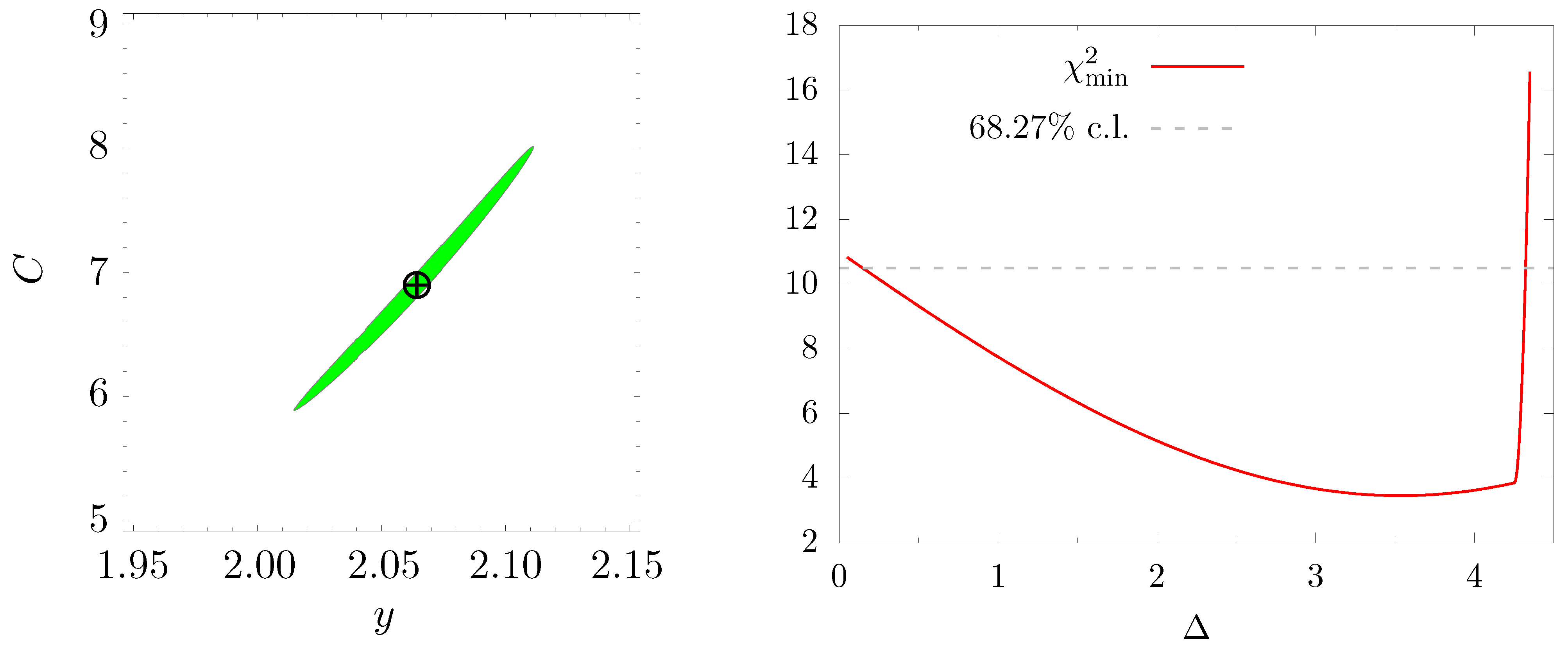
The relatively small uncertainties in the data for $F_{\pi }^2$ and $M_{\pi }^2$, along with the scaling relation $M_{\pi }^2{F}_{\pi }^{2-y}=Cm$, allow for a relatively precise determination of y and C. The correlated $1\sigma$ confidence ranges of these parameters are shown in the left panel of Figure 1, in which the two plots are taken from Ref. [22]. At the $1\sigma$-equivalent confidence level, we found that

$$\begin{array}{c}\hfill y=2.06\pm 0.05.\end{array}$$

(12)

This range of values, if interpreted as the scaling dimension of the chiral condensate of the underlying gauge theory at strong coupling, is consistent with the expectation $y\sim 2$ [9,47,48]. We also found that $f_{\pi }^2/f_d^2=0.086\pm 0.015$.

The ${\chi }^2$ distribution in the full six-dimensional space is relatively flat in the range of $\mathrm{\Delta }$ below $\mathrm{\Delta }\sim 4.25$. The right panel of Figure 1 was obtained by minimizing ${\chi }^2$ of the other five parameters for each given value of $\mathrm{\Delta }$. The curve evolves slowly below $4.25$, with values in the range of $3-4$ being moderately preferred. The flatness of the curve is due, in part, to the lesser accuracy of the lattice data for $M_d^2$. The fit comfortably allows both the marginal deformation case of $|4-\mathrm{\Delta }|\ll 1$ and the “mass-deformation” case of $\mathrm{\Delta }=2$.

3. Beyond Leading Order

In this section, we describe a simple method for determining the dEFT Lagrangian at higher orders in a low-energy expansion. We first demonstrate how this method may be applied to determine the form of the leading-order dEFT Lagrangian ${\mathcal{L}}_{LO}$ in Equation (1). We then apply the method to determine the dEFT Lagrangian at next-to-leading order (NLO) and comment on the relative size of the NLO corrections. Then, by employing a spurion analysis, we highlight the symmetry properties of the dEFT, which motivated and systematized the method employed to construct the dEFT Lagrangian.

3.1. Method for Constructing the Lagrangian

In Section 2, we reviewed our leading-order (LO) construction of the dEFT [22] and its use to fit the LSD lattice data for the $N_f=8$ gauge theory. The fit made use of the LO Lagrangian in Equations (1)–(4), which was implemented in the regime $\langle \chi \rangle =F_d\gg f_d$. In this regime, which is reached by increasing the parameter $m_{\pi }^2$, the scaling laws (Equations (6)–(8)) insure that the dEFT at LO continues to describe a set of pNGBs and a dilaton, each of which is relatively light. The form and estimates of the NLO corrections that we present hold when $F_d\gg f_d$, but we find it simplest to restrict attention to values of $m_{\pi }^2$ for which $F_d$ remains close to $f_d$. Our discussion is then entirely in terms of the lower-case parameters $f_d^2,m_d^2,f_{\pi }^2$, and $m_{\pi }^2$.

The leading-order (LO) Lagrangian density in Equation (1) consists of terms with one power of the squared masses $m_d^2$, $m_{\pi }^2$, or two derivatives ${\partial }^2$. The latter generate contributions of order $p^2$ to observables. Each such factor is taken to be small compared to a natural cutoff $\mathrm{\Lambda }$, which is associated with the masses of heavier physical states when $m_{\pi }^2=0$, which are not included in the dEFT. The dEFT Lagrangian can be described as an expansion in the small, dimensionless combinations $p^2/{\mathrm{\Lambda }}^2$, $m_{\pi }^2/{\mathrm{\Lambda }}^2$, and $m_d^2/{\mathrm{\Lambda }}^2$, which are truncated at some given order.

We first observe that the LO terms themselves can be generated in this manner when combined with a single fine tuning. We begin with a “zeroth-order” Lagrangian density of the form

$${\mathcal{L}}_0=\lambda {\chi }^4,$$

(13)

where $\lambda$ is a dimensionless coefficient taken to be of order ${\mathrm{\Lambda }}^2/f_d^2$ [49]. We then introduce the following set of dimensionless operators.

$$\begin{array}{cccc}\hfill X_1& ={\left(\frac{\chi }{f_d}\right)}^{-2}\frac{{\partial }_{\mu }}{\mathrm{\Lambda }}\left(\frac{\chi }{f_d}\right),\hfill & \hfill X_2& ={\left(\frac{\chi }{f_d}\right)}^{-1}\frac{{\partial }_{\mu }\mathrm{\Sigma }}{\mathrm{\Lambda }},\hfill \\ \hfill X_3& =\frac{m_d^2}{{\mathrm{\Lambda }}^2}{\left(\frac{\chi }{f_d}\right)}^{\mathrm{\Delta }-4},\hfill & \hfill X_4& =\frac{m_{\pi }^2}{{\mathrm{\Lambda }}^2}{\left(\frac{\chi }{f_d}\right)}^{y-4}{\mathbf{1}}_{N_f},\hfill \end{array}$$

(14)

the form of which will be discussed further in the context of a spurion analysis in Section 3.3.

Starting from ${\mathcal{L}}_0$, we construct a series expansion in these operators, retaining only contributions that are Lorentz invariant. Thus, the $X_1$ and $X_2$ operators appear only in pairs. We also use relations of the type

$$1=\frac{1}{N_f}\mathrm{Tr}\left[\mathrm{\Sigma }{\mathrm{\Sigma }}^{†}\right],{\mathbf{1}}_{N_f}=\mathrm{\Sigma }{\mathrm{\Sigma }}^{†},$$

(15)

and then replace $\mathrm{\Sigma }$ (and/or ${\mathrm{\Sigma }}^{†}$) with $X_2$ or $X_4$. Terms in ${\mathcal{L}}_{LO}$ (and then ${\mathcal{L}}_{NLO}$) are also generated by replacing unity with $X_1$ or $X_3$.

Each of the terms in ${\mathcal{L}}_{LO}$, with the important exception of the first term in $V_{\mathrm{\Delta }}$, which is shown in Equation (3), can be generated in this way. The dilaton kinetic term is obtained, up to an $O\left(1\right)$ normalization constant, by replacing unity in ${\mathcal{L}}_0$ with two factors of $X_1$. The pNGB kinetic term Equation (2) is similarly obtained by using Equation (15) and replacing $\mathrm{\Sigma }$ and ${\mathrm{\Sigma }}^{†}$ with $X_2$ and $X_2^{†}$. The pNGB mass term Equation (4) comes, up to an $O\left(1\right)$ factor, from the replacement of unity in ${\mathcal{L}}_0$ with the first relation in Equation (15), the replacement of one factor of $\mathrm{\Sigma }$ with $X_4$, and the addition of the Hermitian conjugate. Here, we take $f_{\pi }^2$ to be of order $f_d^2/N_f$, a value supported by fits to lattice data for the $N_f=8$ theory.

Turning to the potential $V_{\mathrm{\Delta }}$ (Equation (3)), we first note that the two terms are normalized such that for any value of $\mathrm{\Delta }$, the parameters $f_d$ and $m_d^2$ denote the potential minimum and its curvature at the minimum. The limit $\mathrm{\Delta }\to 4$ is smooth. The second term comes from replacing unity in ${\mathcal{L}}_0$ with $X_3$, and it is small relative to ${\mathcal{L}}_0$ for $\mathrm{\Delta }$ not close to 4. Finally, and very critically, the first term is already present in ${\mathcal{L}}_0$, but also in $V_{\mathrm{\Delta }}$ with a coefficient suppressed relative to ${\mathrm{\Lambda }}^2/f_d^2$ when $\mathrm{\Delta }$ is not close to 4. Thus, a single, familiar fine tuning is required to bring this term into line with the others in ${\mathcal{L}}_{LO}$. The full expression for $V_{\mathrm{\Delta }}$ is small relative to ${\mathcal{L}}_0$ for any value of $\mathrm{\Delta }$.

3.2. The dEFT at NLO

We next construct the NLO Lagrangian from ${\mathcal{L}}_{LO}$ in Equation (1) by using the method introduced in Section 3.1. Each NLO-Lagrangian operator is generated by taking each term from ${\mathcal{L}}_{LO}$ and making one replacement with $X_3$ or $X_4$, or two replacements with $X_1$ or $X_2$ from Equation (14). Thus, each NLO operator is quadratic in combinations of $m_{\pi }^2$, $m_d^2$, and paired derivatives, and it also contains a factor $1/{\mathrm{\Lambda }}^2$. We exclude operators that are parity odd. We also remove operators that are rendered redundant by the equations of motion at LO or are proportional to total derivatives. By convention, where there are redundancies, we retain the operators with the fewest derivatives.

The NLO Lagrangian contains three kinds of terms, which we group together as follows:

$${\mathcal{L}}_{NLO}={\mathcal{L}}_{\pi }+{\mathcal{L}}_{p_d}+{\mathcal{L}}_{m_d}.$$

(16)

The first group of terms, ${\mathcal{L}}_{\pi }$, contains factors of $m_{\pi }^2$ and derivatives of the $\mathrm{\Sigma }$ field, but no factors of $m_d^2$ or derivatives of the dilaton field:

$$\begin{array}{cc}\hfill {\mathcal{L}}_{\pi }& =l_0\mathrm{Tr}\left[{\partial }_{\mu }\mathrm{\Sigma }{\partial }_{\nu }{\mathrm{\Sigma }}^{†}{\partial }^{\mu }\mathrm{\Sigma }{\partial }^{\nu }{\mathrm{\Sigma }}^{†}\right]+l_1{\left(\mathrm{Tr}\left[{\partial }_{\mu }\mathrm{\Sigma }{\partial }^{\mu }{\mathrm{\Sigma }}^{†}\right]\right)}^2+l_2\mathrm{Tr}\left[{\partial }_{\mu }\mathrm{\Sigma }{\partial }_{\nu }{\mathrm{\Sigma }}^{†}\right]\mathrm{Tr}\left[{\partial }^{\mu }\mathrm{\Sigma }{\partial }^{\nu }{\mathrm{\Sigma }}^{†}\right]\hfill \\ & +l_3\mathrm{Tr}\left[{\partial }_{\mu }\mathrm{\Sigma }{\partial }^{\mu }{\mathrm{\Sigma }}^{†}{\partial }_{\nu }\mathrm{\Sigma }{\partial }^{\nu }{\mathrm{\Sigma }}^{†}\right]+l_4{m}_{\pi }^2{\left(\frac{\chi }{f_d}\right)}^{y-2}\mathrm{Tr}\left[{\partial }_{\mu }\mathrm{\Sigma }{\partial }^{\mu }{\mathrm{\Sigma }}^{†}\right]\mathrm{Tr}\left[\mathrm{\Sigma }+{\mathrm{\Sigma }}^{†}\right]\hfill \\ & +l_5{m}_{\pi }^2{\left(\frac{\chi }{f_d}\right)}^{y-2}\mathrm{Tr}\left[{\partial }_{\mu }\mathrm{\Sigma }{\partial }^{\mu }{\mathrm{\Sigma }}^{†}\left(\mathrm{\Sigma }+{\mathrm{\Sigma }}^{†}\right)\right]+l_6{m}_{\pi }^4{\left(\frac{\chi }{f_d}\right)}^{2y-4}{\left(\mathrm{Tr}\left[\mathrm{\Sigma }+{\mathrm{\Sigma }}^{†}\right]\right)}^2\hfill \\ & +l_7{m}_{\pi }^4{\left(\frac{\chi }{f_d}\right)}^{2y-4}{\left(\mathrm{Tr}\left[\mathrm{\Sigma }-{\mathrm{\Sigma }}^{†}\right]\right)}^2+l_8{m}_{\pi }^4{\left(\frac{\chi }{f_d}\right)}^{2y-4}\mathrm{Tr}\left[{\mathrm{\Sigma }}^2+{\mathrm{\Sigma }}^{†2}\right]+h_2{m}_{\pi }^4{\left(\frac{\chi }{f_d}\right)}^{2y-4}.\hfill \end{array}$$

(17)

Using the method of replacements from Section 3.1, we estimate that each of the dimensionless coefficients $l_i$ and $h_2$ has a size of order $f_d^2/\left(N_f^t{\mathrm{\Lambda }}^2\right)$, where the power t counts the number of traces taken in the corresponding operator. It can be seen from Equation (15) that each trace comes with a factor of $1/N_f$. The presence of the $m_{\pi /d}^2/{\mathrm{\Lambda }}^2$ and $p^2/{\mathrm{\Lambda }}^2$ factors ensures the smallness of these terms relative to the LO Lagrangian.

To illustrate how the terms in Equation (17) are generated and how the operator coefficients are estimated by using the replacement rules, we consider the first term with coefficient $l_0$ as an example. This operator can be generated starting from the pNGB kinetic term in Equation (2) and inserting $\mathrm{\Sigma }{\mathrm{\Sigma }}^{†}$ inside the trace by using Equation (15). Then, the factor of $\mathrm{\Sigma }$ may be replaced with $X_2$, and ${\mathrm{\Sigma }}^{†}$ with $X_2^{†}$. Contracting the Lorentz indices in one specific way yields the first term in Equation (17). An independent contraction of the Lorentz indices is possible, and is shown as the fourth term with coefficient $l_3$. The order of magnitude of $l_0$ follows directly, without further fine tuning, since the above replacement method multiplies the coefficient $f_{\pi }^2$ in the pNGB kinetic term by $1/{\mathrm{\Lambda }}^2$. One has $l_0\sim f_{\pi }^2/{\mathrm{\Lambda }}^2\sim f_d^2/\left(N_f{\mathrm{\Lambda }}^2\right)$. The natural sizes of the other coefficients in ${\mathcal{L}}_{\pi }$ are estimated in a similar way.

The terms in ${\mathcal{L}}_{\pi }$ are in one-to-one correspondence with those of an EFT for pNGBs without a dilaton, as shown for general $N_f$ in Ref. [50]. The exponent of the dilaton field in each term is determined by the method of replacement, accounting for the constraints imposed by scale invariance. The form of these terms was derived before in Refs. [42,51]. When $N_f=2$ or 3, trace identities relate some of the operators in Equation (17), leading to further simplifications.

The cutoff $\mathrm{\Lambda }$ was estimated in the EFT for pNGBs by calculating the counterterms needed to renormalize the EFT at the one-loop level. The estimates [49,52] indicate that

$${\mathrm{\Lambda }}^2\sim \frac{{\left(4\pi f_{\pi }\right)}^2}{N_f}.$$

(18)

From this, and the expectation $f_{\pi }^2\sim f_d^2/N_f$, the order-of-magnitude estimates for coefficients $l_i$ and $h_2$ can be simplified to

$$l_i,h_i\sim \frac{N_f^{2-t}}{{\left(4\pi \right)}^2}.$$

(19)

We checked that these estimates for the coefficients are consistent with those obtained from the counterterms appearing in Refs. [42,50].

The next group of terms in Equation (16) all contain derivatives of the dilaton field, but no factors of $m_d^2$. The non-redundant set of such terms shown below was also found in Refs. [42,51].

$$\begin{array}{cc}{\mathcal{L}}_{p_d}\hfill & =g_1\frac{{\left({\partial }_{\mu }\chi \right)}^4}{{\chi }^4}+g_2\frac{{\left({\partial }_{\mu }\chi \right)}^2}{{\chi }^2}\mathrm{Tr}\left[{\partial }_{\nu }\mathrm{\Sigma }{\partial }^{\nu }{\mathrm{\Sigma }}^{†}\right]+g_3\frac{{\partial }_{\mu }\chi {\partial }_{\nu }\chi }{{\chi }^2}\mathrm{Tr}\left[{\partial }^{\mu }\mathrm{\Sigma }{\partial }^{\nu }{\mathrm{\Sigma }}^{†}\right]\hfill \\ & +g_4{m}_{\pi }^2{\left(\frac{\chi }{f_d}\right)}^{y-2}\frac{{\left({\partial }_{\mu }\chi \right)}^2}{{\chi }^2}\mathrm{Tr}\left[\mathrm{\Sigma }+{\mathrm{\Sigma }}^{†}\right]+g_5{m}_{\pi }^2{\left(\frac{\chi }{f_d}\right)}^{y-2}\frac{i}{2}\mathrm{Tr}\left[{\partial }_{\mu }\mathrm{\Sigma }-{\partial }_{\mu }{\mathrm{\Sigma }}^{†}\right]\frac{{\partial }^{\mu }\chi }{\chi }.\hfill \end{array}$$

(20)

The $g_i$ coefficients also have a size given by $g_i\sim f_d^2/\left(N_f^t{\mathrm{\Lambda }}^2\right)$ and Equation (19).

Finally, we are left with the group of terms that contain factors of $m_d^2$. They are given by:

$$\begin{array}{c}{\mathcal{L}}_{m_d}=c_1\frac{m_d^2}{(4-\mathrm{\Delta })}\left(1-\frac{4}{\mathrm{\Delta }}{\left(\frac{f_d}{\chi }\right)}^{4-\mathrm{\Delta }}\right){\left(\frac{\chi }{f_d}\right)}^2\mathrm{Tr}\left[{\partial }_{\mu }\mathrm{\Sigma }{\partial }^{\mu }{\mathrm{\Sigma }}^{†}\right]\hfill \\ +c_2\frac{m_d^2{m}_{\pi }^2}{(4-\mathrm{\Delta })}\left(1-\frac{4}{\mathrm{\Delta }}{\left(\frac{f_d}{\chi }\right)}^{4-\mathrm{\Delta }}\right){\left(\frac{\chi }{f_d}\right)}^y\mathrm{Tr}\left[\mathrm{\Sigma }+{\mathrm{\Sigma }}^{†}\right]\\ \hfill +c_3\frac{m_d^4}{{(4-\mathrm{\Delta })}^2}{\left(\frac{\chi }{f_d}\right)}^4{\left(1-\frac{4}{\mathrm{\Delta }}{\left(\frac{f_d}{\chi }\right)}^{4-\mathrm{\Delta }}\right)}^2.\end{array}$$

(21)

Each of the structures above is constructed as a linear combination of an interaction already appearing in ${\mathcal{L}}_{LO}$ and the result obtained by replacing a factor of unity from that interaction with $X_3$. The coefficients of the two pieces are chosen so that each structure contains at least one factor of the following expression:

$$\begin{array}{c}\hfill \frac{m_d^2}{(4-\mathrm{\Delta })}\left(1-\frac{4}{\mathrm{\Delta }}{\left(\frac{f_d}{\chi }\right)}^{4-\mathrm{\Delta }}\right).\end{array}$$

We choose the two terms and the factor of $1/(4-\mathrm{\Delta })$ so that it is a smooth but non-vanishing function of $\chi /f_d$ in the limit $\mathrm{\Delta }\to 4$, as is ${\mathcal{L}}_{LO}$. We also include, as a convention, the weighting factor $4/\mathrm{\Delta }$, reflecting its defining presence in ${\mathcal{L}}_{LO}$1. The sizes of $c_i$ are also given by Equation (19). We are finally left with a total of 18 new operators appearing in the NLO Lagrangian. The full NLO theory, therefore, has a total of $18+6=24$ free parameters.

3.3. Spurion Analysis

By construction, the dEFT is endowed with approximate, spontaneously broken dilatation and internal symmetries. The weak, explicit breaking of these symmetries can be implemented in the dEFT by incorporating spurions into the EFT Lagrangian and including all of the terms allowed by symmetry considerations. In this section, we will employ a spurion analysis to show how the replacement rules (introduced in Section 3.1) emerge and construct the dEFT Lagrangian at LO and NLO.

A spurion is a non-dynamical field that transforms in a given representation of the symmetry group, but then breaks these symmetries once it is assigned a VEV. Since the spurion is not a dynamical field, this introduces explicit rather than spontaneous symmetry breaking. As the appearance of spurions is associated with the presence of the small, dimensionless parameters that control the dEFT expansion, operators in the Lagrangian containing more spurions make contributions to observables that are of a higher order in our dEFT expansion, and they are suppressed once the spurions have been assigned their VEVs.

As with any EFT, we can build the dEFT by employing spurion fields without a detailed description of the underlying gauge theory. We infer the number and symmetry properties of the spurions by comparison with low-energy (lattice) measurements. Once the spurions are chosen, we include all invariant and non-redundant operators at each order in the dEFT expansion. Beyond leading order, observables receive contributions from Feynman diagrams with loops, which can be UV divergent. This procedure will find all the counterterms needed to renormalize the theory, provided that there are no additional sources of symmetry breaking introduced during renormalization.

To allow the dilaton to have mass $m_d^2$ even when the NGBs are massless, we introduce a spurion $\mathcal{S}\left(x\right)$ to break the scale invariance without breaking the internal symmetry. Under dilatations $x\to e^{\rho }x$, it transforms according to

$$\mathcal{S}\left(x\right)\to e^{\rho (4-\mathrm{\Delta })}\mathcal{S}\left(e^{\rho }x\right).$$

(22)

It is assigned to a representation of the dilatation symmetry group labeled by the scaling dimension $4-\mathrm{\Delta }$, which we take to be a free parameter. We measured $\mathrm{\Delta }$ for a specific underlying theory by comparing with lattice data, as described in Section 2.2.

We introduce a second spurion $\mathcal{M}\left(x\right)$ to break the internal symmetry (as well as the scale invariance) and give the pNGBs a mass. It transforms under dilatations according to the rule

$$\mathcal{M}\left(x\right)\to e^{\rho (4-y)}\mathcal{M}\left(e^{\rho }x\right),$$

(23)

where the scaling dimension $4-y$ is interpreted as a free parameter to be determined from low-energy data. We define the spurion field to transform as a conjugate bifundamental field under the unitary transformations $U_{L,R}\in SU{\left(N_f\right)}_{L,R}$:

$$\mathcal{M}\left(x\right)\to U_R\mathcal{M}\left(x\right)U_L^{†}.$$

(24)

Under dilatations, the $\chi$ field transforms with a scaling dimension of one so that $\chi \left(x\right)\to e^{\rho }\chi \left(e^{\rho }x\right)$, whereas the pNGB field transforms with a scaling dimension of zero so that $\mathrm{\Sigma }\left(x\right)\to \mathrm{\Sigma }\left(e^{\rho }x\right)$. Other dimensionful constants that characterize the theory, such as $\mathrm{\Lambda }$ or $f_d$, are left unchanged by this transformation.

We construct operators by using the spurions from which the dEFT Lagrangian density is built. We require each operator:

• to be invariant under Lorentz and internal symmetries,
• to transform with a scaling dimension of 4 under dilatations; the action will then be invariant under dilatations,
• to be polynomial in the spurions and in derivatives.

Crucially, the operators are not required to be polynomial in the dilaton field. Therefore, we introduce the combination $\chi /f_d$ as a conformal compensator and incorporate it within operators raised to noninteger powers2 as necessary to make the operator transform with an overall scaling dimension equal to 4 under dilatations.

To express the LO and NLO Lagrangians in terms of the spurion fields, we employ the replacement method that was already described, but with the $X_3$ and $X_4$ operators of Equation (14) re-expressed as

$$X_3^{sp}=\frac{\mathcal{S}}{{\mathrm{\Lambda }}^2}{\left(\frac{\chi }{f_d}\right)}^{\mathrm{\Delta }-4},X_4^{sp}=\frac{{\mathcal{M}}^{†}}{{\mathrm{\Lambda }}^2}{\left(\frac{\chi }{f_d}\right)}^{y-4}.$$

(25)

It can be seen that the operators $X_1$ and $X_3^{sp}$ are invariant under dilatations and internal symmetry transformations. Similarly, it can be seen that the operators $X_2$ and $X_4^{sp}$ are scale invariant, but transform in the same way as $\mathrm{\Sigma }$ under internal symmetry transformations. It then follows that all valid operators entering ${\mathcal{L}}_{NLO}$ (meaning that they meet requirements 1–3) with increasing powers of $\mathcal{S}$, $\mathcal{M}$, and more derivatives may be generated from operators entering ${\mathcal{L}}_{LO}$ by replacing factors of unity with $X_1$ or $X_3^{sp}$ and factors of $\mathrm{\Sigma }$ with $X_2$ or $X_4^{sp}$. By using this replacement scheme and the relation $\mathrm{\Sigma }{\mathrm{\Sigma }}^{†}={\mathbf{1}}_{N_f}$, all valid operators entering ${\mathcal{L}}_{NLO}$ can be generated.

Once we assign fixed values for the spurions so that they no longer transform, as in Equations (22)–(24), the Lagrangian will explicitly break the dilatation and internal symmetries. We set $\mathcal{S}\to m_d^2$ and $\mathcal{M}\to m_{\pi }^2{\mathbf{1}}_{N_f}$. Setting the $\mathcal{M}$ spurion to be proportional to the identity matrix ensures that the diagonal subgroup $SU{\left(N_f\right)}_V\subset SU{\left(N_f\right)}_L\times SU{\left(N_f\right)}_R$ of the internal symmetry is preserved. Giving all $N_f$ Dirac fermions identical masses in an underlying gauge theory also breaks the internal symmetry in this way. Once the spurions have been assigned their fixed values, the $X_i^{sp}$ operators become their corresponding $X_i$ operators, which take the forms introduced in Equation (14).

4. Summary and Discussion

We have reviewed the features and implementation of the dEFT. We deployed it to provide a continuum description of results from lattice studies of an $SU\left(3\right)$ gauge theory with $N_f$ Dirac fermions in the fundamental representation, but the dEFT itself is universal, and would describe any theory with the same symmetries and pattern of symmetry breaking at sufficiently low energies.

We first summarized in Section 2 the form of the dEFT Lagrangian at leading order (LO) in Equations (1)–(4). It contains a dilaton field associated with the spontaneous breaking of scale invariance in the underlying gauge theory and a set of pNGB fields associated with the spontaneous breaking of the global internal symmetry of the gauge theory. The spontaneously broken scale invariance is also broken explicitly by a relatively small amount. Similarly, the spontaneously broken internal global symmetry is broken explicitly by a pNGB mass $m_{\pi }^2$ needed to compare dEFT predictions with lattice studies.

We then examined the scaling properties of the dEFT, noting that with $m_{\pi }^2$ increased to the values required to describe the lattice data, the explicit breaking of the dilatation and internal symmetries of the dEFT remains small compared to the scale of spontaneous breaking. To this end, the LO Lagrangian was recast in terms of physical (capitalized) quantities in Equations (9)–(11).

In Section 3, we examined the structure of the dEFT at next-to-leading (NLO) order. We developed a “replacement method” for identifying dEFT Lagrangian terms at a given order from those at one order lower. We first demonstrated that the LO Lagrangian itself can be generated in this way starting from the “zeroth-order” Lagrangian in Equation (13). As a next step, the method led to the NLO Lagrangian of Equations (17), (20) and (21). It comprises terms that are generated at the one-loop level and that are naturally suppressed relative to the LO terms. Among the terms of the NLO Lagrangian, some were discussed in our earlier Ref. [22], and most appeared in recent publications [42,51], but some are new. Finally, we motivated the replacement method by showing that it can be derived from a spurion analysis, and we checked that its power-counting matches the loop expansion in the dEFT. Composite Higgs models have been built [23,24] by using dEFT as a foundation, and in this context, NLO interactions modify real-world Higgs boson properties.

Recent lattice studies of nearly conformal gauge theories provide us with a new opportunity to test longstanding but elusive ideas about spontaneously broken scale invariance in quantum field theory, including the hypothesized dilaton. As a greater variety of more precise lattice data become available, it will be important to develop the dEFT further to test the idea. In particular, this requires the systematic calculation of all contributions at NLO to the observables studied on the lattice, including one-loop diagrams. Furthermore, greater theoretical control over lattice artifacts will be needed. This can be achieved by incorporating the symmetry-breaking effects that arise from the lattice discretization within the dEFT itself.

References

- Migdal, A.A.; Shifman, M.A. Dilaton Effective Lagrangian in Gluodynamics. Phys. Lett. 1982, 114B, 445. [Google Scholar] [CrossRef]
- Coleman, S. Aspects of Symmetry: Selected Erice Lectures; Cambridge University Press: Cambridge, UK, 1998. [Google Scholar] [CrossRef]
- Goldberger, W.D.; Grinstein, B.; Skiba, W. Distinguishing the Higgs boson from the dilaton at the Large Hadron Collider. Phys. Rev. Lett. 2008, 100, 111802. [Google Scholar] [CrossRef] [PubMed] [Green Version]
- Leung, C.N.; Love, S.T.; Bardeen, W.A. Spontaneous Symmetry Breaking in Scale Invariant Quantum Electrodynamics. Nucl. Phys. B 1986, 273, 649. [Google Scholar] [CrossRef]
- Bardeen, W.A.; Leung, C.N.; Love, S.T. The Dilaton and Chiral Symmetry Breaking. Phys. Rev. Lett. 1986, 56, 1230. [Google Scholar] [CrossRef] [PubMed]
- Yamawaki, K.; Bando, M.; Matumoto, K.i. Scale Invariant Technicolor Model and a Technidilaton. Phys. Rev. Lett. 1986, 56, 1335. [Google Scholar] [CrossRef]
- Aoki, Y. et al. [LatKMI Collaboration] Light composite scalar in eight-flavor QCD on the lattice. Phys. Rev. D 2014, 89, 111502. [Google Scholar] [CrossRef] [Green Version]
- Appelquist, T.; Brower, R.; Fleming, G.; Hasenfratz, A.; Jin, X.; Kiskis, J.; Neil, E.; Osborn, J.; Rebbi, C.; Rinaldi, E.; et al. Strongly interacting dynamics and the search for new physics at the LHC. Phys. Rev. D 2016, 93, 114514. [Google Scholar] [CrossRef] [Green Version]
- Aoki Y. et al. [LatKMI Collaboration] Light flavor-singlet scalars and walking signals in Nf = 8 QCD on the lattice. Phys. Rev. D 2017, 96, 014508. [Google Scholar] [CrossRef] [Green Version]
- Gasbarro, A.D.; Fleming, G.T. Examining the Low Energy Dynamics of Walking Gauge Theory. PoS Lattice 2017, 2016, 242. [Google Scholar] [CrossRef]
- Appelquist, T. et al. [Lattice Strong Dynamics Collaboration] Nonperturbative investigations of SU(3) gauge theory with eight dynamical flavors. Phys. Rev. D 2019, 99, 014509. [Google Scholar] [CrossRef] [Green Version]
- Appelquist, T. et al. [Lattice Strong Dynamics (LSD)] Goldstone boson scattering with a light composite scalar. Phys. Rev. D 2022, 105, 034505. [Google Scholar] [CrossRef]
- Hasenfratz, A. Emergent strongly coupled ultraviolet fixed point in four dimensions with 8 Kähler-Dirac fermions. arXiv 2022, arXiv:2204.04801. [Google Scholar] [CrossRef]
- Fodor, Z.; Holland, K.; Kuti, J.; Nogradi, D.; Schroeder, C.; Wong, C.H. Can the nearly conformal sextet gauge model hide the Higgs impostor? Phys. Lett. B 2012, 718, 657. [Google Scholar] [CrossRef] [Green Version]
- Fodor, Z.; Holland, K.; Kuti, J.; Mondal, S.; Nogradi, D.; Wong, C.H. Toward the minimal realization of a light composite Higgs. PoS Lattice 2015, 2014, 244. [Google Scholar] [CrossRef] [Green Version]
- Fodor, Z.; Holland, K.; Kuti, J.; Mondal, S.; Nogradi, D.; Wong, C.H. Status of a minimal composite Higgs theory. PoS Lattice 2016, 2015, 219. [Google Scholar] [CrossRef] [Green Version]
- Fodor, Z.; Holland, K.; Kuti, J.; Nogradi, D.; Wong, C.H. The twelve-flavor β-function and dilaton tests of the sextet scalar. EPJ Web Conf. 2018, 175, 08015. [Google Scholar] [CrossRef] [Green Version]
- Fodor, Z.; Holland, K.; Kuti, J.; Wong, C.H. Tantalizing dilaton tests from a near-conformal EFT. PoS Lattice 2019, 2018, 196. [Google Scholar] [CrossRef]
- Fodor, Z.; Holland, K.; Kuti, J.; Wong, C.H. Dilaton EFT from p-regime to RMT in the ϵ-regime. PoS Lattice 2020, 2019, 246. [Google Scholar] [CrossRef]
- Appelquist, T.; Ingoldby, J.; Piai, M. Dilaton EFT Framework For Lattice Data. J. High Energy Phys. 2017, 2017, 035. [Google Scholar] [CrossRef]
- Appelquist, T.; Ingoldby, J.; Piai, M. Analysis of a Dilaton EFT for Lattice Data. J. High Energy Phys. 2018, 2018, 039. [Google Scholar] [CrossRef] [Green Version]
- Appelquist, T.; Ingoldby, J.; Piai, M. Dilaton potential and lattice data. Phys. Rev. D 2020, 101, 075025. [Google Scholar] [CrossRef] [Green Version]
- Appelquist, T.; Ingoldby, J.; Piai, M. Nearly Conformal Composite Higgs Model. Phys. Rev. Lett. 2021, 126, 191804. [Google Scholar] [CrossRef] [PubMed]
- Appelquist, T.; Ingoldby, J.; Piai, M. Composite two-Higgs doublet model from dilaton effective field theory. Nucl. Phys. B 2022, 983, 115930. [Google Scholar] [CrossRef]
- Hong, D.K.; Hsu, S.D.H.; Sannino, F. Composite Higgs from higher representations. Phys. Lett. B 2004, 597, 89. [Google Scholar] [CrossRef] [Green Version]
- Dietrich, D.D.; Sannino, F.; Tuominen, K. Light composite Higgs from higher representations versus electroweak precision measurements: Predictions for CERN LHC. Phys. Rev. D 2005, 72, 055001. [Google Scholar] [CrossRef] [Green Version]
- Hashimoto, M.; Yamawaki, K. Techni-dilaton at Conformal Edge. Phys. Rev. D 2011, 83, 015008. [Google Scholar] [CrossRef] [Green Version]
- Appelquist, T.; Bai, Y. A Light Dilaton in Walking Gauge Theories. Phys. Rev. D 2010, 82, 071701. [Google Scholar] [CrossRef] [Green Version]
- Vecchi, L. Phenomenology of a light scalar: The dilaton. Phys. Rev. D 2010, 82, 076009. [Google Scholar] [CrossRef] [Green Version]
- Chacko, Z.; Mishra, R.K. Effective Theory of a Light Dilaton. Phys. Rev. D 2013, 87, 115006. [Google Scholar] [CrossRef]
- Bellazzini, B.; Csaki, C.; Hubisz, J.; Serra, J.; Terning, J. A Higgslike Dilaton. Eur. Phys. J. C 2013, 73, 2333. [Google Scholar] [CrossRef] [Green Version]
- Bellazzini, B.; Csaki, C.; Hubisz, J.; Serra, J.; Terning, J. A Naturally Light Dilaton and a Small Cosmological Constant. Eur. Phys. J. C 2014, 74, 2790. [Google Scholar] [CrossRef] [PubMed] [Green Version]
- Abe, T.; Kitano, R.; Konishi, Y.; Oda, K.y.; Sato, J.; Sugiyama, S. Minimal Dilaton Model. Phys. Rev. D 2012, 86, 115016. [Google Scholar] [CrossRef] [Green Version]
- Eichten, E.; Lane, K.; Martin, A. A Higgs Impostor in Low-Scale Technicolor. arXiv 2012, arXiv:1210.5462. [Google Scholar]
- Hernandez-Leon, P.; Merlo, L. Distinguishing A Higgs-Like Dilaton Scenario With A Complete Bosonic Effective Field Theory Basis. Phys. Rev. D 2017, 96, 075008. [Google Scholar] [CrossRef] [Green Version]
- Matsuzaki, S.; Yamawaki, K. Dilaton Chiral Perturbation Theory: Determining the Mass and Decay Constant of the Technidilaton on the Lattice. Phys. Rev. Lett. 2014, 113, 082002. [Google Scholar] [CrossRef] [Green Version]
- Golterman, M.; Shamir, Y. Low-energy effective action for pions and a dilatonic meson. Phys. Rev. D 2016, 94, 054502. [Google Scholar] [CrossRef] [Green Version]
- Kasai, A.; Okumura, K.i.; Suzuki, H. A dilaton-pion mass relation. arXiv 2016, arXiv:1609.02264. [Google Scholar]
- Hansen, M.; Langaeble, K.; Sannino, F. Extending Chiral Perturbation Theory with an Isosinglet Scalar. Phys. Rev. D 2017, 95, 036005. [Google Scholar] [CrossRef] [Green Version]
- Golterman, M.; Shamir, Y. Effective pion mass term and the trace anomaly. Phys. Rev. D 2017, 95, 016003. [Google Scholar] [CrossRef] [Green Version]
- Golterman, M.; Shamir, Y. Large-mass regime of the dilaton-pion low-energy effective theory. Phys. Rev. D 2018, 98, 056025. [Google Scholar] [CrossRef] [Green Version]
- Cata, O.; Muller, C. Chiral effective theories with a light scalar at one loop. Nucl. Phys. B 2020, 952, 114938. [Google Scholar] [CrossRef]
- Catà, O.; Crewther, R.J.; Tunstall, L.C. Crawling technicolor. Phys. Rev. D 2019, 100, 095007. [Google Scholar] [CrossRef] [Green Version]
- Golterman, M.; Neil, E.T.; Shamir, Y. Application of dilaton chiral perturbation theory to Nf = 8, SU(3) spectral data. Phys. Rev. D 2020, 102, 034515. [Google Scholar] [CrossRef]
- Golterman, M.; Shamir, Y. Explorations beyond dilaton chiral perturbation theory in the eight-flavor SU(3) gauge theory. Phys. Rev. D 2020, 102, 114507. [Google Scholar] [CrossRef]
- Leung, C.N.; Love, S.T.; Bardeen, W.A. Aspects of Dynamical Symmetry Breaking in Gauge Field Theories. Nucl. Phys. B 1989, 323, 493–512. [Google Scholar] [CrossRef]
- Cohen, A.G.; Georgi, H. Walking Beyond the Rainbow. Nucl. Phys. B 1989, 314, 7–24. [Google Scholar] [CrossRef]
- Ryttov, T.A.; Shrock, R. Higher-order scheme-independent series expansions of and β′IR in conformal field theories. Phys. Rev. D 2017, 95, 105004. [Google Scholar] [CrossRef] [Green Version]
- Georgi, H. Generalized dimensional analysis. Phys. Lett. B 1993, 298, 187–189. [Google Scholar] [CrossRef] [Green Version]
- Bijnens, J.; Lu, J. Technicolor and other QCD-like theories at next-to-next-to-leading order. J. High Energy Phys. 2009, 11, 116. [Google Scholar] [CrossRef]
- Li, Y.L.; Ma, Y.L.; Rho, M. Chiral-scale effective theory including a dilatonic meson. Phys. Rev. D 2017, 95, 114011. [Google Scholar] [CrossRef] [Green Version]
- Soldate, M.; Sundrum, R. Z Couplings to Pseudogoldstone Bosons Within Extended Technicolor. Nucl. Phys. B 1990, 340, 1–32. [Google Scholar] [CrossRef]
Figure 1.
The 1 ranges for the scaling dimensions y and , as defined in the main body of the paper, obtained in fits of LSD lattice measurements in the theory with fundamental fermions [22].
Disclaimer/Publisher’s Note: The statements, opinions and data contained in all publications are solely those of the individual author(s) and contributor(s) and not of MDPI and/or the editor(s). MDPI and/or the editor(s) disclaim responsibility for any injury to people or property resulting from any ideas, methods, instructions or products referred to in the content. |
© 2022 by the authors. Licensee MDPI, Basel, Switzerland. This article is an open access article distributed under the terms and conditions of the Creative Commons Attribution (CC BY) license (https://creativecommons.org/licenses/by/4.0/).
Share and Cite
MDPI and ACS Style
Appelquist, T.; Ingoldby, J.; Piai, M. Dilaton Effective Field Theory. Universe 2023, 9, 10. https://doi.org/10.3390/universe9010010
AMA Style
Appelquist T, Ingoldby J, Piai M. Dilaton Effective Field Theory. Universe. 2023; 9(1):10. https://doi.org/10.3390/universe9010010
Chicago/Turabian StyleAppelquist, Thomas, James Ingoldby, and Maurizio Piai. 2023. "Dilaton Effective Field Theory" Universe 9, no. 1: 10. https://doi.org/10.3390/universe9010010
Note that from the first issue of 2016, this journal uses article numbers instead of page numbers. See further details here.