

Abstract
Seagrass meadows globally are under pressure with worldwide loss and degradation, but there is a growing recognition of the global importance of seagrass ecosystem services, particularly as a major carbon sink and as fisheries habitat. Estimates of global seagrass spatial distribution differ greatly throughout the published literature, ranging from 177 000 to 600 000 km2 with models suggesting potential distribution an order of magnitude higher. The requirements of the Paris Climate Agreement by outlining National Determined Contributions (NDC's) to reduce emissions is placing an increased global focus on the spatial extent, loss and restoration of seagrass meadows. Now more than ever there is a need to provide a more accurate and consistent measure of the global spatial distribution of seagrass. There is also a need to be able to assess the global spread of other seagrass ecosystem services and in their extension, the values of these services. In this study, by rationalising and updating a range of existing datasets of seagrass distribution around the globe, we have estimated with Moderate to High confidence the global seagrass area to date as 160 387 km2, but possibly 266 562 km2 with lower confidence. We break this global estimate down to a national level with a detailed analysis of the current state of mapped distribution and estimates of seagrass area per country. Accurate estimates, however, are challenged by large areas remaining unmapped and inconsistent measures being used. Through the examination of current global maps, we are able to propose a pathway forward for improving mapping of this important resource. More accurate measure of global #seagrass distribution, critical for assessing current state and trends
Export citation and abstract BibTeX RIS

Original content from this work may be used under the terms of the Creative Commons Attribution 4.0 license. Any further distribution of this work must maintain attribution to the author(s) and the title of the work, journal citation and DOI.
1. Introduction and background
Seagrass meadows globally are under pressure and experiencing accelerating degradation due to both direct and indirect human activities and climate change [1]. Although there are some small glimmers of hope [2], this crisis has human consequences, as many hundreds of millions of people directly rely on healthy seagrass ecosystems for their food and livelihood [3, 4]. With growing recognition of the global importance of the ecosystem services provided by seagrass, particularly as a major carbon sink and as fisheries habitat [3, 5], now more than ever there is a need to provide a more accurate and consistent measure of the global spatial distribution of seagrass meadows. This is particularly the case given the recognition of their role in developing nature-based solutions to climate change [6]. With increasing focus on quantifying ecosystem services, whether these are intrinsic or extrinsic, knowledge is required of where seagrass occur as a resource.
Based on previous estimates, seagrasses are reported to occur in 191 countries and across six global bioregions spanning the tropical and temperate seas [7]. Estimates of global seagrass spatial distribution differ greatly throughout the published literature, ranging from 177 000 to 600 000 km2 [8, 9]. In some parts of the world, this is due to limited mapping efforts, but it is also because seagrass meadows are not static (naturally changing in the absence of human activities) and because of the difficulties associated to mapping consistently in many environments that vary in water clarity and depth [10]. The potential area for seagrass to occupy globally, based on the light regime (irradiance reaching the bottom of the coastal ocean), bathymetry, and seagrass light requirements (≥ 5.1 mol photons m−2 d−1), has been estimated to be 4 320 000 km2 [11]. Recent approaches using maximum entropy modelling (MaxEnt) have refined this estimate using species distribution records and environmental variables to estimate the potential area suitable for seagrass globally to be 1 646 788 km2 [12]. Although such models assist with providing estimates of where seagrass might occur, at large scales they may fail to effectively consider the variability in environmental factors, possibly due to the limitation within available data sources, leading to both false positives and false negatives.
The first global synthesis and the most extensive collection of seagrass spatial distribution maps are located at the UNEP World Conservation Monitoring Centre (WCMC) [13]. The result of a 2001 workshop, the global seagrass atlas estimated a composite global seagrass coverage of 177 000 km2 [9]. The dataset (and subsequent versions) was created from multiple sources (e.g. 547 sources across 128 countries and territories), including maps from various times (1930–2015), and of various scales (from 1:1000 e.g. [14] to 1:28 510 000 e.g. [15]). The data also lacked consistency in mapping methods, which varied from qualitative (anecdotal/expert interpolation with no documented/visual evidence) to quantitative, accurate field validation [13]. Nearly two decades have passed since the first global database/atlas was developed and efforts to map the global distribution of seagrass and populate significant data gaps (e.g. insular Southeast Asia, the east coast of South America and the west coast of Africa) appear largely stagnant. Some regions of the world suspected to support vast seagrass meadows remain largely uncharted, for example, the Philippines [16]. Willingness to conserve seagrass can only translate into effective action if informed by where it is found, its condition and threats and its value (in terms of ecosystem services) [17]. In order for seagrass ecosystems to be included in spatial management plans and marine protected areas, it is imperative that we know where they are.
Mapping seagrass needs to consider more than its spatial extent as not all seagrasses are the same, their function and ecosystem service provisioning changing across genera and environmental gradients, therefore we need to characterise seagrass into separate seagrass biotopes so that differential ecosystem service values can be assigned. For example, the value of a dense Enhalus acoroides meadow with a > 1 m high canopy is very different to one based on the small-leaved (< 2 cm high) Halophila ovalis [17–19]. This is important so that if seagrass is to be included in spatial management plans and marine protected areas, it is designated based on the type of ecosystem services that type of meadow provides.
The overall aim of this study was to assess the global spatial distribution of seagrass, which has been done based on rationalising and updating several different existing datasets of seagrass distribution around the globe. Specifically, we provide a detailed analysis of the current state of mapped distribution and estimates globally and for each country seagrass has been reported or likely to occur with levels of confidence. We also discuss the importance of understanding the distribution and abundance of seagrasses globally.
2. Methods
In the present study, we estimated the global area of known seagrass distribution by rationalising and updating various existing datasets of mapped seagrass meadows. We gathered published data using online searches (Google Scholar & Google), freely accessible seagrass data portals, virtual herbaria and authors' personal data collections (figure 1). These data included seagrass meadows ranging in size from a few square meters to thousands of square kilometres. As maps of seagrass distribution can be individual observations (points) or measured areas (polygons or vector-based), for our assessment we exclusively used polygon (vector-based) maps for measures of spatial extent. Point data were used only to indicate seagrass presence.
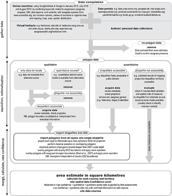
Figure 1. Schematic diagram illustrating the processes of gathering, acquisition, rationalisation, and merging of spatial data for the calculation of seagrass area estimates in each country.
Download figure:
Standard image High-resolution imageFor our estimate of global seagrass area we have used the WCMC database [13] and where available, included additional polygon data in the public domain (e.g. Seamap Australia [20]) or spatial values from published literature where mapping was conducted that resulted in vector-based Geographic Information System (GIS) layers. Polygons of non-seagrass (aquatic plant) genera (e.g. Vallisneria, Najas) were removed from the WCMC dataset [13] before analysis. Where possible, we have also corrected some of the qualitative (anecdotal) polygon data in the WCMC database [13] by rationalising (replacing or removing) data where seagrass presence has been mapped with greater accuracy or not been confirmed based on point records (e.g. herbaria), published literature, or authors knowledge. In situations where polygons from both qualitative (unvalidated opinions) and quantitative (field validated mapping) was available, the field validated mapping took precedence as it was the only evidence-based data. Where a time series of spatial data is available for a country, we have used the composite (maximum compiled extent, sensu [9]), which represents the full spatial extent of all datasets collected. Bathymetry spatial data at 1:10 m scale was accessed from Natural Earth (North American Cartographic Information Society). Exclusive Economic Zones (EEZ) to 200 nmi (nautical miles), including areas in the provisions of the United Nations Convention on the Law of the Sea (UNCLOS), were used to delineate maritime boundaries for each country or territory [21].
Our spatial assessment of available polygon data was conducted using a GIS with ArcMap® software (version 10.4.1). The area of each polygon was calculated in square kilometres in the Mollweide equal area cylindrical WGS-84 projection. As the dataset contained overlapping polygons, a dissolve operation was conducted before area calculations and any polygon portions located deeper than 200 m water depth were erased. The 200 m contour is the shallowest bathymetric depth available globally. Prior to individual country area calculations, polygons were overlaid with EEZ and a union operation applied, i.e. to separate continuous polygons overlapping two or more EEZ boundaries. Similarly, for seagrass bioregional calculations, country area polygons were overlaid with the six global seagrass bioregion boundaries.
Finally, we rated the Confidence level of the merged seagrass area estimated for each country according to the data sources (figure 1). When quantitative and qualitative spatial data was available and supported by field assessments (including point data from herbaria, etc), we classified the data as Moderate to High confidence, i.e. data source is known or derived from supporting evidence (e.g. field validation) and/or expert knowledge [22]. When only qualitative data were available we classified the data as Low confidence, i.e. data source derived from limited expert knowledge with restricted/no history about how data was collected or created [22].
3. Results and discussion
Our analysis estimates the compiled global seagrass area composite to date as 160 387 km2 across 103 countries/territories with Moderate to High confidence, with an additional 106 175 km2 across another 33 countries with Low confidence (table 1). These two combined give an estimate of 266 562 km2. This estimate is near the lower end of the 300 000 to 600 000 km2 range suggested by previous studies [8, 23]. The country with the highest compiled seagrass area was Australia, which at 83 013 km2 (74 579.39 km2 in seagrass bioregion 5 and 8433.59 km2 in seagrass bioregion 6) represents over 31% of global known seagrass area. The country with the lowest seagrass area according to this analysis was Cape Verde at 20 m2 [24].
Table 1. Global distribution of coastal marine habitats and revised estimates of global seagrass area (including confidence) within each seagrass bioregion, including length of coastline and modelled potential seagrass area (MaxEnt). Seagrass bioregions from Short et al (2007). Coastline in kilometres from the World Vector Shoreline (WVS). Modelled (MaxEnt) global distribution of the seagrass biome from Jayathilake and Costello [12].
| Area (km2) | |||||||||||
|---|---|---|---|---|---|---|---|---|---|---|---|
| Seagrass bioregion | Coastline length | MaxEnt (km2) | Moderate—High | Low confidence | Proportion of global | Seagrass area (km2) | |||||
| Habitat | (km) | confidence | total (%) | relative to coastline | |||||||
| Seagrass | length | Latitudinal extent | Area source | ||||||||
| 1. Temperate North Atlantic | 218 243 | 259 384 | 3229 | 1.21 | 0.01 | 70°N–33°N | this study | ||||
| 2. Tropical Atlantic | 54 438 | 297 782 | 44 222 | 65 231 | 41.06 | 2.01 | 33°N–30°S | this study | |||
| 3. Mediterranean | 61 527 | 118 913 | 14 167 | 10 862 | 9.39 | 0.41 | 53°N–20°N | this study | |||
| 4. Temperate North | 106 706 | 127 805 | 1866 | 0.70 | 0.02 | 68°N–20°N | this study | ||||
| 5. Tropical Indo-Pacific | 235 261 | 628 703 | 87 791 | 30 082 | 44.22 | 0.50 | 32°N–29°S | this study | |||
| 6. Temperate Southern Oceans | 47 679 | 172 322 | 9112 | 3.42 | 0.19 | 26°S– 47°S | this study | ||||
| —outside any bioregion | 11 664 | 26 186 | |||||||||
| TOTAL | 735 518 | 1 631 096 | 160 387 | 106 175 | 70°N–47°S | this study | |||||
| Coral reefs | 284 803.00 | 34°N–32°S | |||||||||
| Mangroves | 152 361.00 | 32°N–40°S | |||||||||
| Saltmarsh | 54 950.89 | 76°N–55°S | |||||||||
| Kelp | ∼ 15 000.00 | 80°N–24°N 3°S–56°S | |||||||||
We identified seagrass occurrence in 163 of the 209 countries and territories located within global seagrass bioregions (table 1). Of the 163 countries and territories where seagrass occurrence is confirmed, 17% lacked spatial data (table 1).
In the countries where seagrass occur, they can be a significant component of coastal habitats. Some of the highest national seagrass extents relative to coastline occur in the Caribbean Sea region of the Tropical Atlantic (Region 2) (figure 2). Surrounding the deeper basins of the Caribbean Sea, seagrass are widespread on the shallow shelf surrounding island nations (e.g. Cuba and Antigua & Barbuda) and adjacent to the continental coasts of the Americas (e.g. Mexico and USA). Similarly, in region 5 the seagrass extent relative to coastline is much greater in countries within shallow (< 100 m depth) enclosed seas (e.g. Persian Gulf) or where the continental shelf supports large shallow gulfs (e.g. Sri Lanka and Cambodia) and lagoons (e.g. Great Barrier Reef) (figure 2).
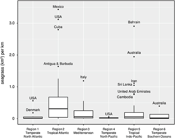
Figure 2. Relative extent of seagrass spatial area mapped with moderate to high confidence, (km2) per kilometre of each country's coastline, within each seagrass bioregion. Note that the coastlines of some countries (e.g. USA and Australia) occur in more than a single seagrass bioregion. The box represents the interquartile range of values, where the boundary of the box closest to zero indicates the 25th percentile, a line within the box marks the median, and the boundary of the box farthest from zero indicates the 75th percentile. Whiskers (error bars) above and below the box indicate the 90th and 10th percentiles, and the dots represent outlying points.
Download figure:
Standard image High-resolution image3.1. Comparable global marine habitat area estimates
In our assessment, we find that the extent of seagrass meadows is conservatively estimated to be higher than mangrove, saltmarsh and kelp habitats, but marginally lower than coral reefs (table 1), although none of the area estimates are considered to be complete. Unlike coral reefs, mangroves and kelp forests, a key feature of seagrass is the occurrence of these communities into temperate and even polar latitudes and the patchiness of the observations.
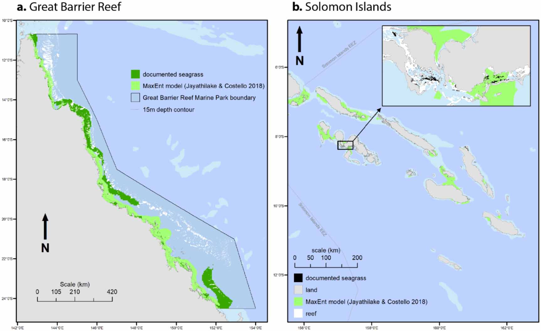
The compiled global seagrass area in our assessment is less than a fifth of the total extent of seagrass predicted using MaxEnt modelling (see table 1). However, approximately 60% of the globally documented seagrass area [13] was not contained (polygon overlay) within the MaxEnt predicted distribution. Closer examination of the MaxEnt model reveals further limitations. For example, on the Great Barrier Reef which includes a range of tropical and subtropical habitats (estuary, coastal, reef, deep-water), and where extensive mapping over the last 30 years has documented 35 679 km2 of seagrass (Australia bioregion 5 in supplement table S1(stacks.iop.org/ERL/15/074041/mmedia)), the MaxEnt model predicted 59 340 km2 of potential seagrass area. Although this may be within the models predictive power (76% more than half the time) on closer examination the differences between the predicted and documented are more concerning. For example, in waters shallower than 15 m, MaxEnt over-predicted seagrass extent by 525%, with 4% of the documented seagrass falling outside prediction area; in waters deeper than 15 m, MaxEnt over-predicted by 21%, but 70% of the documented seagrass was outside the predicted area (figure 3(a)). Similarly, in the Solomon Islands, where seagrasses are predominately restricted to lagoons and narrow fringing reefs, MaxEnt over-predicted the seagrass extent by 850%, but 90% of the documented seagrass was outside the predicted area (figure 3(b)). The Western European distribution of seagrass proposed by the MaxEnt modelling approach also suffers inaccuracies by predicting seagrass to be abundant in many of the region's best surf spots, conditions of which are inappropriate for seagrass. In general, we found the MaxEnt predictions to have no significant relationship to observed seagrass extent (mapped with moderate to high confidence), and that on average MaxEnt values were approximately 17 000 km2 different on average from the linear regression line (figure 4).

Figure 3. MaxEnt model [12] and documented seagrass distribution for (a) Great Barrier Reef, north-eastern Australia [25–27]; (b) Solomon Islands [28, 29].
Download figure:
Standard image High-resolution image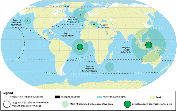
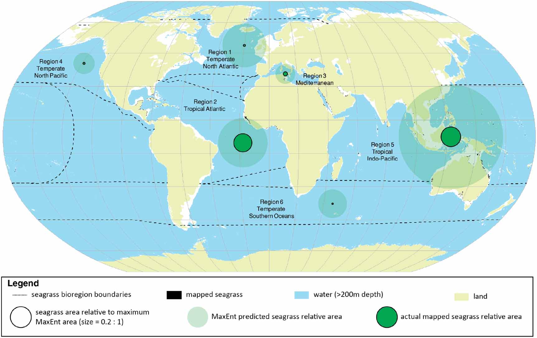
Figure 4. Compiled global seagrass area (mapped, from table S1) relative to the maximum potential seagrass area (modelled with MaxEnt [12]) within each of the global seagrass bioregions. Bioregional seagrass areas represented by scaled circles.
Download figure:
Standard image High-resolution imageAs two of these examples include the range of seagrass habitats and communities present throughout the Indo-Pacific region, it raises concern regarding the use of the MaxEnt model as a surrogate for mapping in data deficient locations across the Pacific Islands and Southeast Asia. It is inevitable that such global-scale modelling assessments will be applied at smaller scales, particularly at the country-wide level. In reality, the current MaxEnt model is useful for identifying the potential regional occurrence of seagrass species, but should not be used for area measurements, particularly regarding blue carbon sink capacity calculations.
Although this does not negate such modelling attempts, it does indicate 'room for improvement'. The model may be more appropriate if applied using a higher level of probability (e.g. 0.8 or 0.95), however, this was beyond the scope of the present study. Not only are models only as good as the input data on which they are based (e.g. bathymetry (depth resolution), substrate type (including grain size and consolidation) and hydrodynamic processes (level of shelter from waves or benthic shear)), but also modellers need to work more closely with ecologists to ensure meaningful findings.
3.2. Considerations and recommendations for the global dataset
3.2.1. Accuracy, level of confidence and consistency
All maps include an element of map error [30]. Without knowledge of the mapping method and some measure of error, it is not possible to decide whether a map is fit for purpose [31]. Different mapping approaches will map different levels of spatial or thematic detail [32]. Given their importance, it is critical to understand the reliability and accuracy of area estimates. This is a key element missing from the global database which can have significant consequences, e.g. spatial ecosystem service valuation [33]. It is also important that the original mapping scale is available in global datasets as this provides some indication of confidence. For example, data sources in the global database include not-to-scale hand-drawn sketch maps where the data accuracy is often overlooked by the general user (figure 5).

Figure 5. Example of data migration from 'not drawn to scale' sketch to GIS: (a) hand-drawn source (reprinted from [34], copyright (1989), with permission from Elsevier) (note 'not drawn to scale'); (b) digitised into WCMC database, and; (c) revised polygons from 'to scale' surveys. On average, meadows in 'not drawn to scale' source extended 10 km from shoreline, however in 'to scale' survey, meadows rarely extended greater than 1 km from shoreline.
Download figure:
Standard image High-resolution imageWe estimate that of the 136 countries for which spatial data was available, 40% of the data could be classified as Low confidence (table 1). One of the data sources identified within the WCMC database [13] was from the global coral reef map [15] (approx. 60% of the data). The origin of the seagrass maps presented within the global coral reef map [15] were not-to-scale hand-drawn sketches from anecdotal information which generally overestimate seagrass presence and extent. For example, the area of seagrass in the Solomon Islands from the global coral reef map [15] was 1262 km2, however, remote sensing overlaid with field surveys reported 66 km2 [28]; a 19 fold difference. Similarly, in Hawaii (USA), the global coral reef map [15] polygon area was 596 km2, however, the documented area is actually 0.02 km2 [35]; a near 30 000 fold difference. Although these mapping inconsistencies and inaccuracies should not discount the WCMC database [13], they do highlight the need to acknowledge the inaccuracies (i.e. use with caution), consistency and need to improve the global dataset.
The global dataset needs to contain fields which provide additional information such as accuracy, description of data capture methods and possibly values to quantify the error around the area estimate. For this dataset to have greater value, approaches will also need to be considered when datasets of variable accuracy are processed at each step of the mapping process to accommodate the propagation of errors into the final map. Routine integration of disparate datasets would also need to be facilitated by the use of robust and repeatable methods at the collection and map creation stages.
3.2.2. Limitations
Knowing where seagrasses do not occur is also critical for a broad range of economic valuations, human impact assessments, and for the development of policy, planning and management (including restoration) in coastal areas. Existing global datasets rarely distinguish 'no data' from 'no seagrass' (e.g. species occurrence databases such as the Ocean Biogeographic Information System (OBIS) [36, 37]). Many areas which are devoid of seagrass may simply be areas for which there are no observations (e.g. vast areas of South East Asia). This also includes limited mapping efforts in turbid water systems and in some geographic regions that have received less attention from the scientific community or local government agencies [38].
Also, consideration should be given to measures such as seagrass density, to enable tracking of global trends beyond only distribution [39]. This, however, may necessitate the acknowledgement that abundance should be included as a direct measure of conservation importance, similar to coral reef health. This additional information will be critical for estimating global carbon budgets and designing Marine Protected Area networks.
3.2.3. Additional data sources
Of the 163 countries and territories we confirmed seagrass occurrence, 17% lacked spatial data. There exists a critical need to develop consistent global mapping approaches and bring disparate datasets into a single common platform, to provide a foundation for a global observing network [39]. This could be through support of an existing or alternative portal. Unfortunately, not all researchers and/or agencies contribute data to the existing WCMC database. This has often been the result of data not being linked to a published report or scientific publication. However, issues of data ownership and intellectual recognition, as well as long-term stewardship, and universal and equitable access to, quality-assured scientific data and data services, products, and information are now overcome with online data archiving and publishing organisations (e.g. The World Data Center PANGAEA®). Reliable (quality) high-resolution (e.g. 1:10 000 scale) seagrass maps should be identified and accessed from other sources where possible. These may be located from scientific publications or within National data repositories, e.g. Seamap Australia, Lembaga Ilmu Pengetahuan Indonesia (LIPI, Indonesia). These maps may include a variety of spatial scales, which we recommend be constrained within the patch to regional meadow scales to be of most value for ecosystem valuations and conservation planning.
3.2.4. Challenges in mapping seagrass
Many of the world's seagrass areas remain uncharted even at a high level of spatial and thematic detail. For example, we identified 27% of countries within seagrass bioregions lack data (i.e. presence or absence could not be confirmed). This is mostly a consequence of seagrass' submerged characteristic in deep and/or turbid water, and an inability to differentiate low to moderate seagrass from the often dark unconsolidated substrate. However, technological advances in recent years have improved our ability to identify and characterise seagrasses from other benthos.
Nevertheless, seagrass mapping is still not without its challenges mostly due to the difficulty in visually identifying features. Environmental conditions such as turbidity and water depth within the coastal zone are highly variable in space and/or time, making the observation of seagrass challenging. Next to that, seagrasses vary in shape, composition, abundance, biomass and complexity (e.g. 10% cover of Halophila ovalis with 4 cm canopy height vs 10% Enhalus with 1 m canopy height) versus a variety of background of unconsolidated material (e.g. terrigenous sand vs carbonated sand). It is for these reasons that mapping seagrass around the world remains a challenge [10]. For example, despite a long history of marine science in the United Kingdom, seagrass remains poorly mapped, where many of these challenges come into play, particularly the common presence of turbid waters restricting seagrass observations.
Seagrasses are naturally highly dynamic and seasonal, making quantifying their distribution fraught with variability [40]. The complexity of the habitat (e.g. patchiness, algal or coral-seagrass mix) and its variable density further adds additional challenges, particularly for seagrass in low density or for species with low relative biomass [10].
Validating seagrass occurrence can also be challenging because of difficulties associated with remote inaccessibility (limited to where people or robots can go). In remote parts of the Indian Ocean deep-water seagrasses are likely extensive, yet very poorly mapped [41]. In such instances, interpolations from limited field assessments are required.
Finally, the poor prioritization afforded to seagrass, and their often extensive latitudinal spread, means that the appropriate resources required to conduct the mapping are rarely made available [16].
3.3. Rising to the challenge of mapping the worlds seagrass distribution
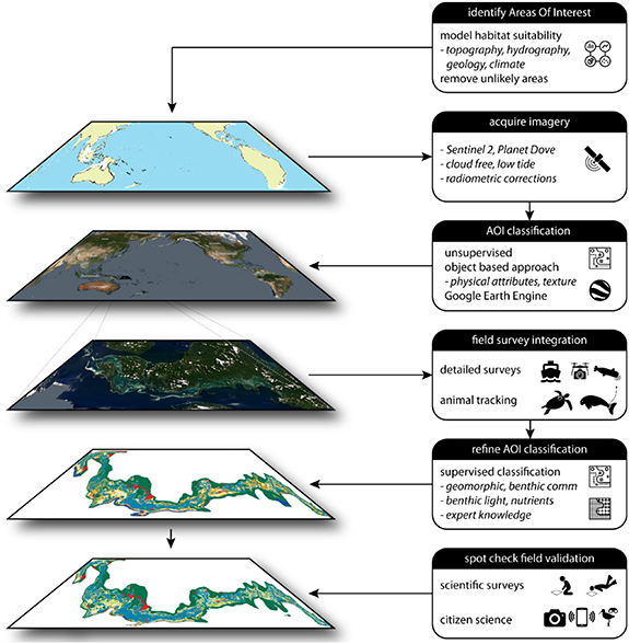
In order to improve the mapping of the world's seagrass distribution, we need to update and rationalise current resources so that seagrass stakeholders globally can see gaps and develop appropriate priorities and targets accordingly. Current efforts are underway to address the inaccuracies and completeness in many maps but these efforts need to be extended [42]. We propose that an hierarchical mapping approach, such as used for parts of the Great Barrier Reef and Pacific Islands, can be applied globally (figure 6). It includes combining eco-geomorphological principles and hierarchical object-based analysis to create mapping rules using various input data layers, which are then coupled with field validation data from an assortment of sources.
Figure 6. Hypothetical example for mapping the world's seagrass using hierarchical approach.
Download figure:
Standard image High-resolution image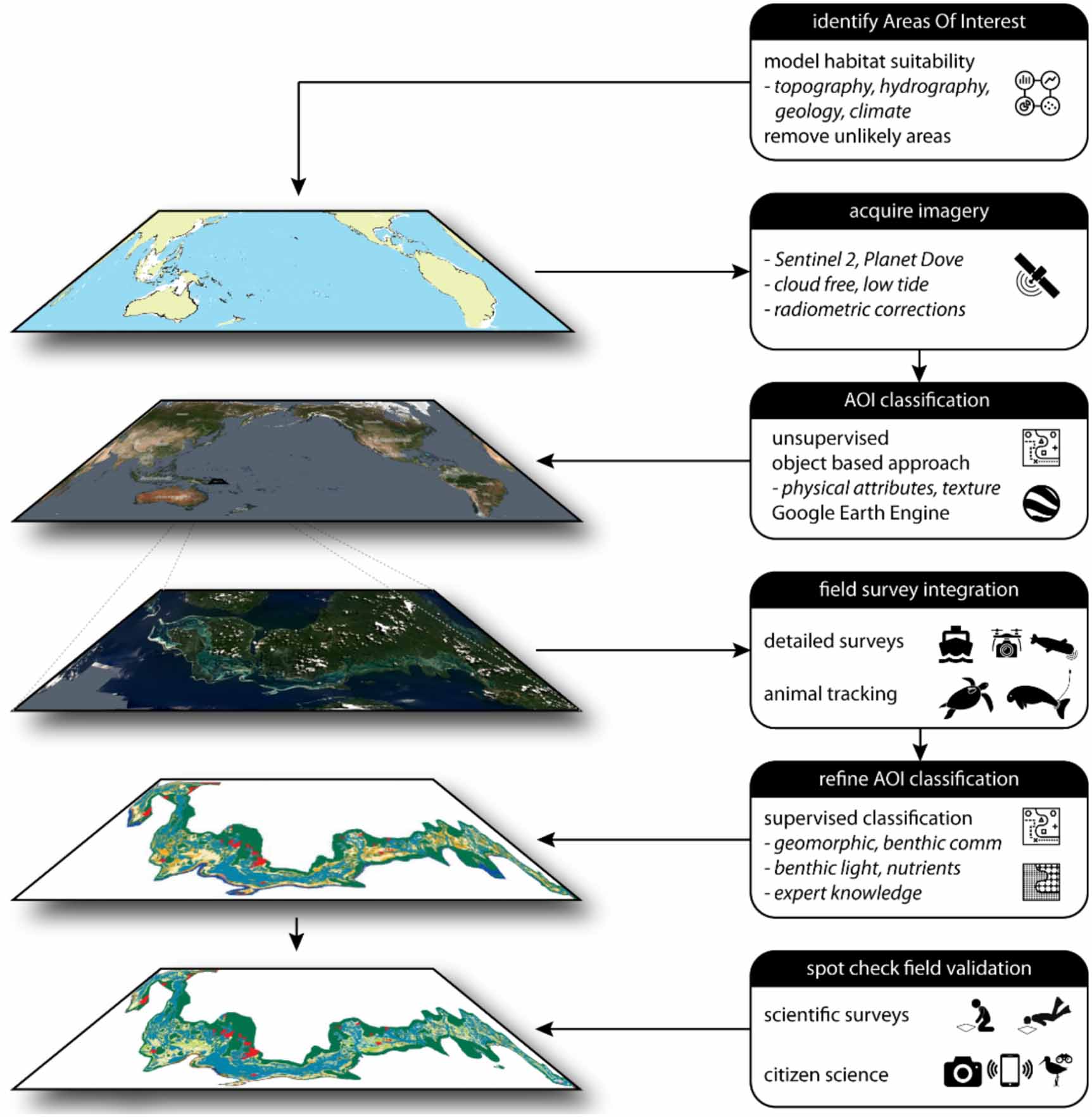
The use of remote air-borne or satellite sensors enables many areas of shallow water (< 8 m depth) seagrass to be rapidly mapped, although use of such technology can become problematic in complex multi-habitat seascapes, murky or deeper waters [30]. It is for this reason that we also need to move towards new innovative approaches in order to fill this vast spatial knowledge gap in our understanding of global seagrass. Improvements in the spatial, spectral and temporal resolution of satellite remote sensing platforms such as Copernicus Sentinel-2 [43] and Planet Dove [44] are helping to fill gaps. The increasing accessibility to high-quality drone sensors is also enhancing the environmental window of opportunity for the use of such methods for observing and quantifying seagrass for smaller areas at a high level of detail [45]. Development of object-based analysis approaches can increase the capability to map seagrass as has been done for coral reefs [46]. These use not only the individual pixel colour of the satellite image within objects, but also its texture or shape of object, or the location of an object in relation to other objects, next to physical attribute known to influence seagrass growth such as depth, slope consolidation [47].
The increase in high spatial and temporal imagery provides the unique ability to join data sets to strengthen mapping protocols, this together with online processing capability such as with Google Earth Engine platform will provide another opportunity to better assess seagrass extent globally. Initial trials for the Greek territorial waters have shown some success using this approach with Copernicus Sentinel-2 for clear waters and structurally large seagrass species (e.g. Posidonia) [48], however extensive methods and accuracy testing across a variety of habitats and seagrass communities are required.
In deeper waters (> 8 m depth), autonomous underwater vehicles (AUVs or robots) and remotely operated underwater vehicles (ROVs) offer new possibilities to collect visual data across large spatial areas [49], expanding our knowledge of where seagrass exist [50]. Similarly, improvements in the use of side-scan and multi-beam sonar [51] can improve mapping resolution, which although promising for mapping structurally large seagrasses [51, 52], find smaller and sparser seagrass difficult to detect [53]. Nevertheless, these acoustic tools can assist in benthic habitat characterization by providing improved bathymetry and sediment type predictions that can also be used to interpret benthic shear stress and tidal currents [54], which potentially could be used to extrapolate mapping efforts and improve identification of potential seagrass areas. Discovery of new seagrass areas in remote localities commonly off the conservation radar can also be aided by novel approaches such as the tagging of migratory mega-herbivores [55].
Finally, more simplistic mechanisms such as the greater engagement of citizen scientists [56] also offer solutions to help map or validate maps. Using novel approaches such as crowdsourcing with smartphone apps including SeagrassSpotter, or content analysis of geo-tagged photographs from freely accessible photo-sharing platforms such as Flickr is proving highly successful in not only identifying seagrass presence but also providing key information on seagrass species and phenology [57]. Additionally, the ability to collect geo-tagged photo-quadrats and analyse them semi-automatically for benthic composition [58] for tens of thousands of photos is standard verification in large scale habitat coral reef habitat mapping and could potentially be applied to seagrass [59]. Alternatively, collaborating with well-established citizen science programs examining seagrass associated fauna may provide valuable information. For example, wetland birdwatching is a popular activity globally, where observations are uploaded to online databases (e.g. birdlife.org.au, ebird.org) with real-time data about bird distribution, abundance and their habitats [60] may provide an untapped resource.
The solutions presented to address the challenge are not exhaustive, and as new technologies are realised (e.g. machine learning, AI), creative problem-solving hackathons may provide an opportunity to develop novel tools and techniques (hacks/workarounds) for streamlining data acquisition and analysis at higher resolution in real-time.
4. Conclusions
The requirements of the Paris Climate Agreement by outlining National Determined Contributions (NDC's) to reduce emissions is placing an increased global focus on the spatial extent, loss and restoration of seagrass meadows. In this study, we find that seagrass is globally extensive and to date 160 387 km2 has been mapped across 103 countries with Moderate to High confidence, with an additional 106 175 km2 mapped across another 33 countries with Low confidence. In conclusion, our extent value falls well short of modelled estimates of where seagrass could be and interrogations of these maps shows how countries such as the Philippines, Indonesia, Russia and Canada that are known to contain seagrass remain inadequately mapped and in many other countries mapped areas are likely only a small proportion of what exists. As a priority, we recommend that seagrass distribution data (GPS coordinates and shapefiles on seagrass extent) that already exists to be archived (with appropriate spatial data agreements) in a centralised global GIS clearinghouse, such as the World Conservation and Monitoring Centre. Open access of seagrass distribution data along with more accurate and consistent measure of the global spatial distribution of seagrass is key to successful seagrass conservation. This distribution information is urgently needed for examining the global contribution of seagrass carbon stocks in global carbon models and to more accurately monitor seagrass loss and gain.
Acknowledgments
We thank Helen Kettles (Department of Conservation, New Zealand), Lauren Weatherdon (UNEP-WCMC), and Rudi Yoshida (Seagrass-Watch) for their assistance with data gathering. We also thank Lucas Langlois (JCU) for his assistance with figure 2. We sincerely thank the two anonymous reviewers for the time they spent on the careful reading of our manuscript and their many insightful comments and suggestions. LMN acknowledges funding from the Swedish Research Council Formas (Grant No. 2014-1288).
Data availability statement
The data that underpin the analysis within this study were mostly sourced from publically available online data portals. In locations where we were unable to access original shapefiles of seagrass extent we have used values provided in relevant publications, all sources used in this paper are cited. Unfortunately, we are not permitted to share the shapefiles produced in this paper due to restrictions on distribution to third party. We strongly urge everyone with seagrass distribution data to publish those on publically available open access platforms.
Author contributions
Study was conceived by all authors. LJM conducted the analyses and created figures. LMN, LJM, and RKFU lead the writing. All authors have contributed to the development and writing of the manuscript and given approval of the final version of the manuscript.