Automatic Delineation of Forest Patches in Highly Fragmented Landscapes Using Coloured Point Clouds
by
 ,
,
José V. Roces-Díaz
1,† ,
,
Carlos Cabo
1,2,3,*,†,
Covadonga Prendes
2,
Celestino Ordoñez
3 and
Cristina Santín
1,4 1
Department of Geography, College of Science, Swansea University, Wallace Building, Singleton Park, Swansea SA2 8PP, Wales, UK
2
Forest and Wood Technology Research Centre Foundation (CETEMAS), Pumarabule s/n, 33936 Carbayín, Asturias, Spain
3
Department of Mining Exploitation and Prospecting, University of Oviedo, 33003 Oviedo, Spain
4
Department of Biosciences, College of Science, Swansea University, Wallace Building, Singleton Park, Swansea SA2 8PP, Wales, UK
*
Author to whom correspondence should be addressed.
†
Both authors have contributed equally to this manuscript and share first position.
Forests 2020, 11(2), 198; https://doi.org/10.3390/f11020198
Submission received: 8 December 2019
/
Revised: 28 January 2020
/
Accepted: 7 February 2020
/
Published: 11 February 2020
(This article belongs to the Special Issue Characterizing of the Structure and the Species Composition of Forest by Using Multiple Remote Sensing Data Sources or Inventory Approaches)
Abstract
:Accurate mapping of landscape features is key for natural resources management and planning. For this purpose, the use of high-resolution remote sensing data has become widespread and is increasingly freely available. However, mapping some target features, such as small forest patches, is still a challenge. Standard, easily replicable, and automatic methodologies to delineate such features are still missing. A common alternative to automated methods is manual delineation, but this is often too time and resource intensive. We developed a simple and automatic method from freely available aerial light detection and ranging (LiDAR) and aerial ortho-images that provide accurate land use mapping and overcome some of the aforementioned limitations. The input for the algorithm is a coloured point cloud, where multispectral information from the ortho-images is associated to each LiDAR point. From this, four-class segmentation and mapping were performed based on vegetation indices and the ground-elevation of the points. We tested the method in four areas in the north-western Iberian Peninsula and compared the results with existent cartography. The completeness and correctness of our algorithm ranging between 78% and 99% in most cases, and it allows for the delineation of very small patches that were previously underrepresented in the reference cartography.
1. Introduction
Accurate mapping and classification of landscape elements including different land covers (crops, pastures, forest areas, etc.) and ecosystems is key for land planning, natural resources management and biodiversity conservation [1,2,3]. In this sense, over the last few decades, a wide range of products and methodologies related to landscape mapping have been released (e.g., [2,4,5,6,7]). Available products for landscape delineation are mainly derived from remote sensors and cover a range of spatial, temporal and spectral resolutions that affect mapping accuracy [8,9]. For example, high temporal resolution data (i.e., one or more images per year) allow for monitoring ecosystems changes and dynamics (e.g., decline of forest ecosystems related with biotic or abiotic factors). High spectral resolution (i.e., availability of several spectral bands) allows the estimation of different types of indices (e.g., the widely used normalised difference vegetation index, NDVI) in order to support classification and mapping processes [10]. Finally, high spatial resolution images (i.e., pixel sizes smaller than 1–2 m [11]) allow for the delineation of small or very narrow features or patches. Small-sized forest patches, isolated trees, and non-forest woody formations are relevant elements of traditional landscapes of Europe [12]. Thus, their identification and delineation are frequently highlighted as key for the development of sustainable management and conservation tools for rural landscapes [13,14,15].
The manual delineation of features is the most obvious and direct method for mapping small-sized patches (e.g., [16,17]). For this reason, it was the basis for the first highly detailed landscape maps during the twentieth century. Manual delineation is often based on the use of aerial imagery (mainly ortho-images) with very high spatial resolution (typically with pixel sizes of 0.05–0.5 m [17]). However, these types of images are not always available in open repositories. The main limitation of these manual processes for patch delineation and identification is that they are very time consuming and subject to the interpretation of the operators.
Automatic and semi-automatic methods (i.e., typically unsupervised and supervised classifications, respectively) constitute an alternative to manual delineation and are commonly applied to satellite images from different sensors [10] such as Sentinel or Landsat. Although these data often provide higher levels of spectral and temporal resolution than the most common aerial images (i.e., aerial ortho-photographs [11,18]), they have, in general, lower levels of spatial detail. These limitations result in some small patches (or individual features) not being delineated.
Aerial light detection and ranging (LiDAR) provides a less time-consuming alternative to manual delineation. In addition, it provides higher spatial detail than traditional remote sensing imagery as well as information to characterise the spatial structure of the ecosystems (i.e., their height in relation to the ground floor level). Aerial light detection and ranging technologies are already well established and accepted as a useful tool for landscape mapping and classification processes (e.g., [7,19]). This type of dataset is becoming increasingly available. In many European countries, point clouds from their whole territory are available such as the National Air Ortho-photography Programme in Spain (PNOA) [20], Finland [21], Denmark [22] and Poland [23]. Other countries provide free point clouds of all their territories as is the case for the USA [24], Canada [25] and New Zealand [26]. In other world regions, including most of the South and Central Americas and Africa, data capture at the country level is undeveloped. However, several LiDAR studies [18,27,28] show the increasing interest of these countries in this data source. The data from these national LiDAR campaigns is usually provided with some sort of land cover/use classification. These classifications use point cloud geometry as a unique input and, in most cases, are based on a height normalization followed by multiple elevation thresholding and local texture analyses. References in the literature to these methods are numerous [29,30,31,32,33,34], and they often describe the use of existing software (e.g., Terrascan, LasTools, FME, Envi) or combinations of them. One of their main shortcomings is that they fail at differentiating covers with similar local textures and elevations.
In order to overcome some of the abovementioned limitations, our main aim was to develop a simple, automatic, and easily replicable method for mapping and classifying landscape patches using publicly available data: coloured LiDAR point clouds with multispectral data from aerial imagery. Four classes were mapped at very high spatial resolution (2 m pixel size): (i) forests, (ii) shrublands and low vegetation, (iii) buildings, and (iv) bare soil areas.
The developed method was tested in the highly heterogeneous landscape of the NW Iberian Peninsula (Galicia, Spain), and accurately identified different types of patches, particularly those which were woody dominated, included both forests and non-forest woody formations.
2. Materials and Methods
2.1. Study Area for Testing
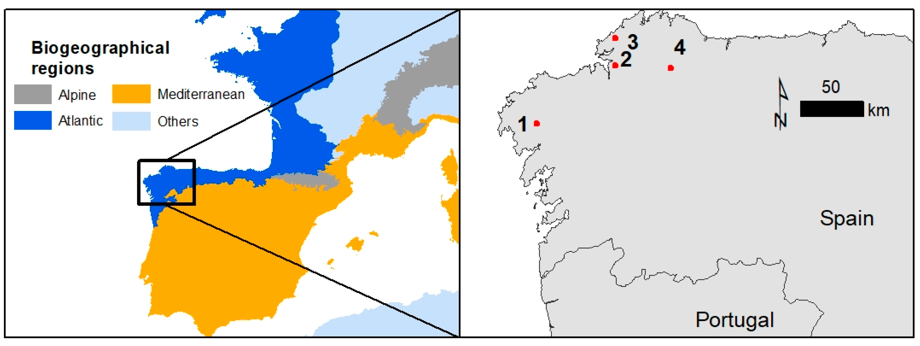
To test our method, we selected four 2 × 2 km study areas located in Galicia, northwest of the Iberian Peninsula, European Atlantic Region (Figure 1). In general, the landscape of this area is highly heterogeneous with a large number of small forest patches combined with multiple types of land uses [35]. The predominant forest vegetation types are deciduous stands (mainly Quercus sp.) mixed with coniferous (Pinus sp.) and eucalypts (Eucalyptus sp.) plantations. On the one hand, the four areas are similar in terms of altitude (an altitude range of 50–250 m over sea level), type of terrain (slopes from moderate to high, between 5% and 35%), and ecological context (i.e., the same biogeographical regions). On the other hand, they show differences regarding landscape composition (e.g., higher values of forest cover in Area 4) and configuration (e.g., more fragmented patches in Area 1). See the results in Section 3.1 for further details.
2.2. Methodological Approach and Type of Data Used
Our algorithm used the LiDAR data available in the PNOA [20], which consist of LAS [36] binary files (the LAS format is used for managing LiDAR point cloud datasets) delivered in 2 × 2 km tiles of coloured point clouds. In addition to the information for the x, y, and z coordinates, every point in the cloud contains colour information from ortho-images in three bands: near infrared (NIr), red (R), and green (G). The data are freely available online in this format for the whole Spanish territory. The NIr sensor used in the data acquisition was a Leica RCD30 [37] which incorporates a monochrome charged coupled device (CCD) which is spectrally separated from the red, green, and blue (RGB) bands through a dichroic beam splitter device; thus, it can be considered as a near infrared-modified camera. In order to create distortion-free images of nominal focal length and pixel size, the NIr band was interpolated to the resolution of RGB. The point cloud and the spectral information were fused using a zenithal projection, so the colour attributes were added to each point in the cloud.
We developed a simple method that takes advantage of the two main aspects/attributes of the data we used: spectral and geometric information. As previously explained, the spectral data provided by coloured point clouds are modified for visualisation purposes and, therefore, not the most suitable for land cover classification. However, the robustness of some vegetation indexes (i.e., NDVI [38]) allows for a simple dichotomous classification (vegetated/non-vegetated land cover) even with this uncalibrated data. The calculation of the elevation of the elements/features on the ground from LiDAR point clouds has been extensively studied in the last two or three decades (e.g., [2,6]). Most of the existing methods generate a terrain model using regular grids or triangulated irregular networks. Once the terrain models are generated, calculating the elevation above them of every point in the original cloud is straightforward.
2.3. Methodology
2.3.1. NDVI-Based Segmentation
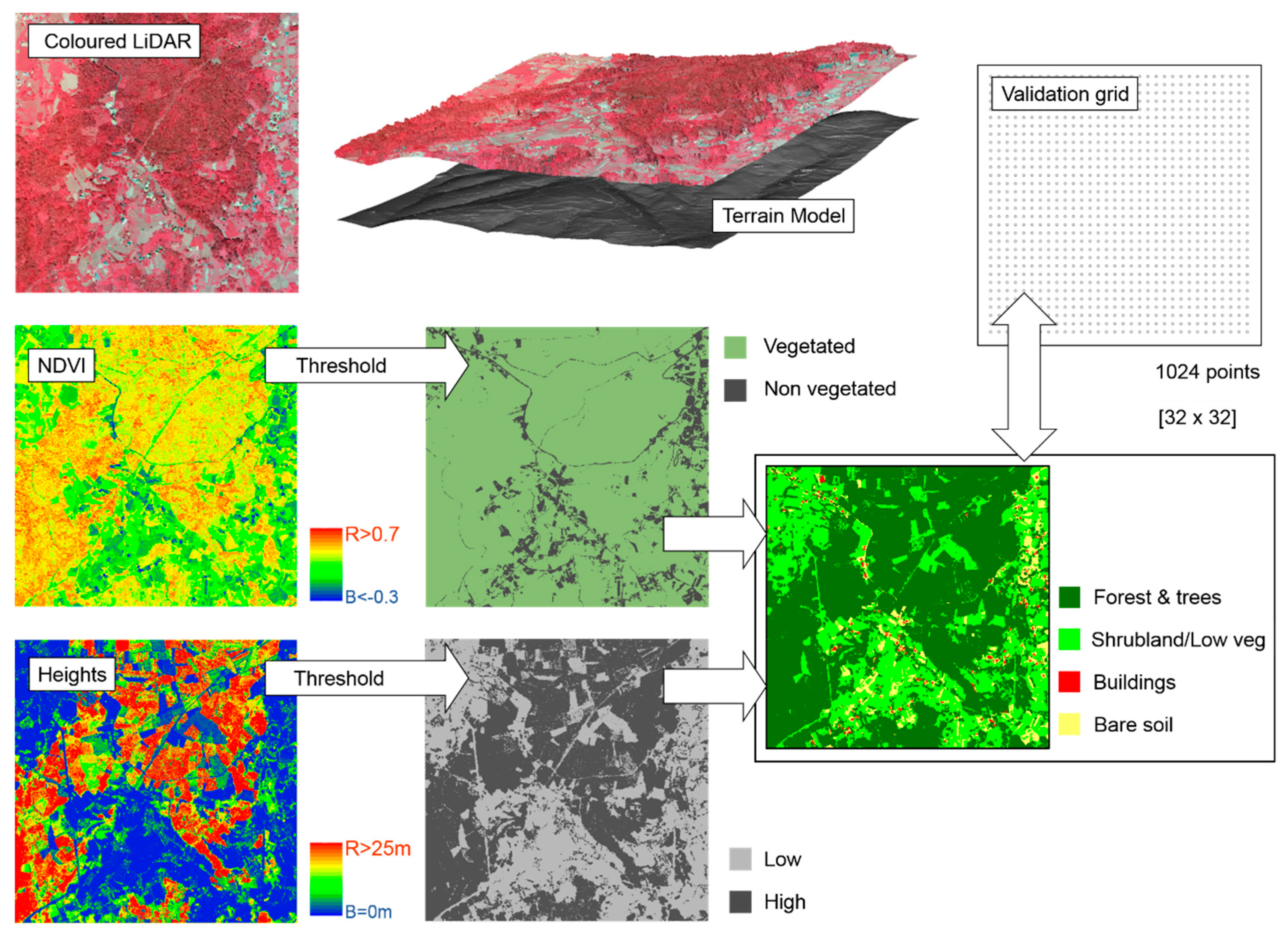
In the first stage of the method, NDVI is computed from NIr and R values [39] for each point. The procedure is implemented through a simple arithmetic operation, and it is performed on a matrix of size n × 2, n being the number of points in the cloud with two columns for R and NIr values. As a result, a new column/field is generated and added to the original point cloud that contains NDVI values, ranging from −1 to 1. Afterwards, points belonging to vegetated versus non-vegetated covers/features are separated by thresholding the NDVI values. This threshold may vary depending on the data source, study area, season, etc., but it is, in general, established in values around NDVI = 0 [40,41]. It is important to highlight that only calibrated NDVI values can be used to compare points in different locations, epochs or datasets; however, when the information is used to determine the distribution of relative variability (as it is in this study) the radiometric calibration of the data is not always indispensable. According to Xu et al. (2014) [41], several studies have obtained good results testing the potential of the near infrared-modified cameras (with ground-based, unmanned aerial vehicle UAV, or other airborne perspectives) to be used without calibration and transformation of the digital numbers (DNs) of the images into reflectance [11,42,43,44]. Figure 2 shows an RBG representation of the NIrRG values, and the result of the NDVI-based thresholding in a 2 × 2 km point cloud tile. For this study, we used a threshold = 0.0 for NDVI values.
2.3.2. Elevation-Based Segmentation
In the second stage of the method, the points from the cloud are height normalized, i.e., the height above the ground of each point is computed by modelling the terrain. The automatic generation of accurate terrain models from aerial point clouds has been tackled from many different perspectives [6]. In this study, we used the Cloth Simulation Algorithm (CSA), developed by Zhang et al. (2016) [45]. The CSA creates a regular grid that covers the whole extent of the point cloud. Then, the nodes of the grid are treated as a cloth with inverted gravity. The result is a cloth-like grid that adapts to the terrain, leaving out the elements that protrude from the terrain such as trees, buildings, or other volumetric structures. The resulting terrain grid (or virtual cloth) is smothered using a Laplacian filter. From this, distances of every point to the cloth are calculated (i.e., elevation of the points from the terrain model). The elevation is added as a new column/field to the original cloud. The same elevation threshold (3 m) was applied in the four test areas. This value represents the general minimum height of trees for this geographical area.
2.3.3. Segmentation and Classification
The original point cloud is subsequently segmented into four target classes. In order to perform this segmentation, threshold values for NDVI and elevation are considered in order to assign a class to each point (see Figure 2). The classification is performed as described in Table 1: (i) points are tagged as “Forest” if they are high (above the elevation threshold) and vegetated (above the NDVI threshold); (ii) “Shrubland or low vegetation” if they are low (below the elevation threshold) and vegetated (above the NDVI threshold); (iii) “Building” if they are high (above the elevation threshold) and non-vegetated (below the NDVI threshold); and (iv) “Bare soil” if they are low (below the elevation threshold) and non-vegetated (below the NDVI threshold). The final result (classified point cloud) is transformed into a raster. The ground sample distance (GSD) of the raster may vary depending on the density of the point cloud, so there is at least one point at the majority (or all) of the positions of the grid/raster (pixels). In cases where several points are at the same position of the grid, a preference rule applies in the following order: (i) forest, (ii) buildings, (iii) shrubland and low vegetation, and (iv) bare soil. In this way, if there are points from different classes in the same pixel, the pixel is tagged as the point of highest order (e.g., if there are “forest” points, the pixel is tagged as so; if not, if there are “building” points, the pixel is tagged as “building”, and so on). If there is a pixel with no points in it, it will be tagged as the majority of its neighbours are in order to fill the possible gaps.
2.4. Validation
We validated our algorithm using a regular grid of 32 × 32 points (n = 1024; distance between consecutive points: 60 m; see Validation grid in Figure 2) for each study area. The class values for each point (ground truth) were extracted from visual inspection of the coloured point clouds by two different operators. We also compared the performances of the algorithm for the four 2 × 2 km study areas with reference cartography from two different reference maps:
- (i)
- Corine Land Cover (CLC18) [46]. This version was updated in 2018. It provides a map of 44 land cover hierarchical classes for all of the European Union with a minimum mapping unit (MMU) of 25 ha and a minimum width of linear elements of 100 m;
- (ii)
- Spanish Forest Map 1:25,000 (SFM25) [47]. This thematic map focuses on forest ecosystems, providing an accurate delineation of tree-dominated ecosystems with multiple applications for forest and land planning at different scales (e.g., [48,49]). The SFM25 has a higher spatial resolution than CLC18 with an optimum pixel size of 10–15 m (according to recommendations in Hengl (2006) [50]) and a MMU ranging from 0.5 to 2 ha). For each landscape polygon delineated, it includes the percentage of tree and shrub cover and the three dominant tree species where these exist.
To compare the three different datasets, we clustered different classes (both in CLC18 and in SFM25) to create new broader classes comparable to those generated by our algorithm. We created a typology of four main classes based on the existence of vegetation cover and the height of the landscape elements. Then, we adapted the legend of the two reference maps to these four classes. For example, some semi-natural areas from CLC18 (i.e., shrublands) were separated from forests and combined with other types of low vegetation. Further information is provided in Table 1. Similarly, we re-classified SFM25 using the information from each individual polygon into the four classes previously mentioned (Table 1).
The performance of the method was measured by calculating confusion matrices (a widely accepted method for performance estimation [51]) from the values in the validation grid and the three datasets: results from the algorithm, CLC18 and SFM25. We computed the completeness and correctness for each class (forest/trees, shrubland, buildings, and bare soil), area, and dataset. Finally, we estimated the total accuracy and the Cohen’s kappa coefficient for our algorithm and for the two reference maps.
Completeness (CM; Equation (1)) provided information about the detection rate, i.e., the proportion of points that were visually assigned to a specific class in the validation grid and were correctly detected.
Correctness (CR; Equation (2)) provided information about the correct classification rate, i.e., the proportion of points from the validation grid that were correctly assigned to the class they belong to.
Accuracy (AC; Equation (3)) provided information about the overall completeness of the method, i.e., the proportion of the total number of points that were correctly assigned to their class.
3. Results
3.1. Delineation of Landscape Elements
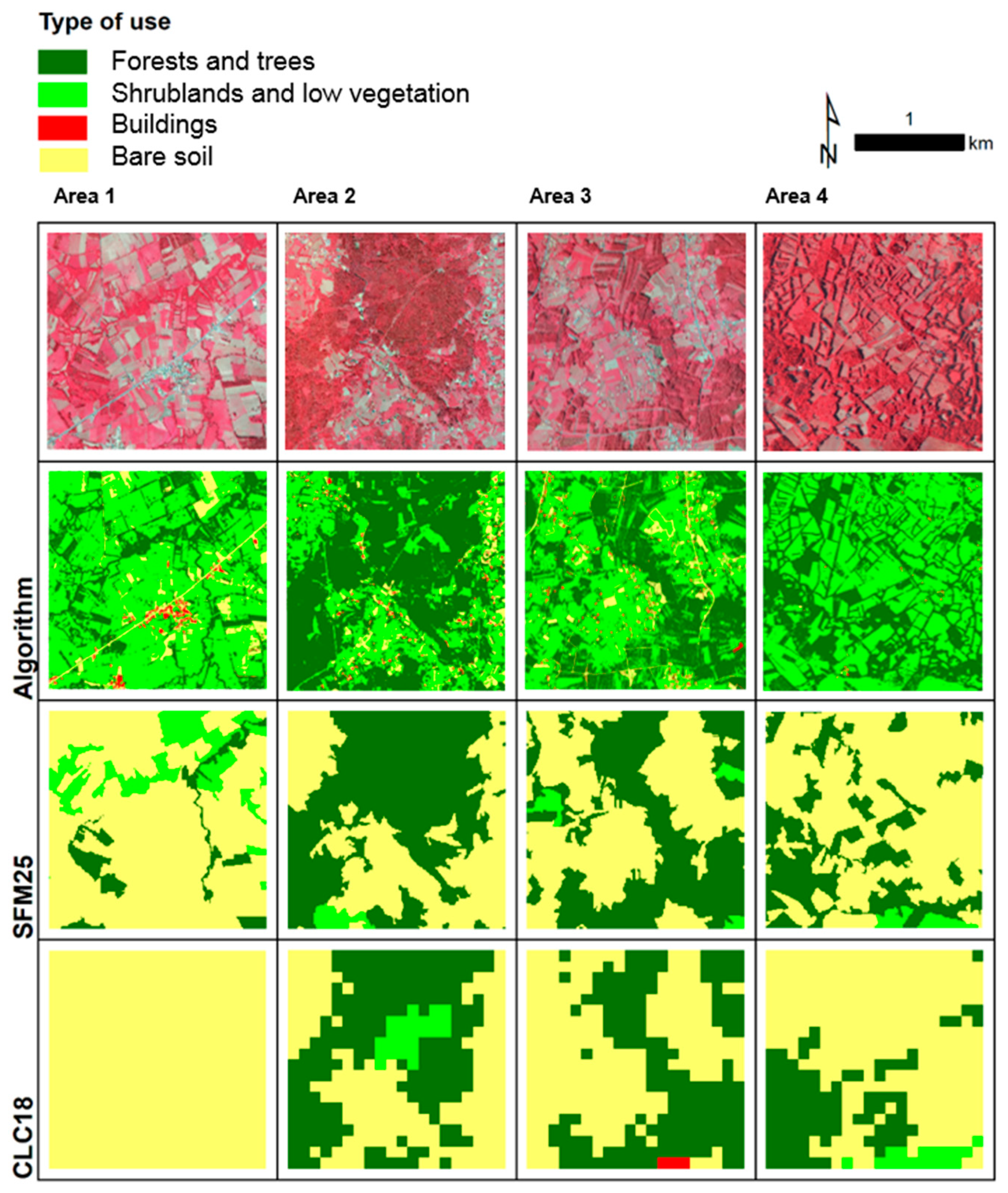
The method proposed here allowed the automatic mapping of the four study areas at high spatial resolution (pixel size 2 × 2 m). The classification of the study areas, which covered 4 km2, only required seconds of data processing using a standard computer. In general, the four study areas show that low vegetation (including shrubs, pastures, and crops) were the dominant cover (40–70%; Figure 3). Forest covered the largest areas with different levels of fragmentation (e.g., larger and more continuous patches in Area 2 and higher fragmentation in Area 4) or shapes (predominant lineal patches in Area 1). Tree patches were scarcer in Area 1 (<20%), where lineal shapes were predominant which represented forested hedgerows and similar structures. Areas covered by buildings and other artificial elements were identified within the four areas but, in general, showed lower cover values.
The delineation derived from the two reference maps (i.e., SFM25 and CLC18) provided different results to those obtained by our algorithm. In general, both datasets showed lower levels of occurrence for areas covered by forest patches in our study cases (lower than 45% except for Area 2). Comparing our findings with SFM25, the delineation of forested areas was similar, although a higher number of linear elements covered by woody vegetation were identified by our algorithm (see for example Area 4 in Figure 3). Our methodology also showed a higher level of performance for detecting woody hedgerows in comparison with CLC18. In fact, the last did not show any forest/tree/vegetation cover for Area 1, meanwhile our algorithm showed a tree cover of <20%. In addition, and in contrast with our algorithm, the two reference maps showed that those areas with bare soil (mainly arable lands) constitute the dominant class (40–70%; Figure 3). Finally, artificial covers (e.g., roads or paved areas) and buildings were practically absent in our study areas (Figure 3), but our algorithm detected existing ones, whereas CLC18 did not detect any (except for some pixels from Area 3), and SFM25 did not include this type of use.
3.2. Validation of Our Results and Comparison with Other Datasets
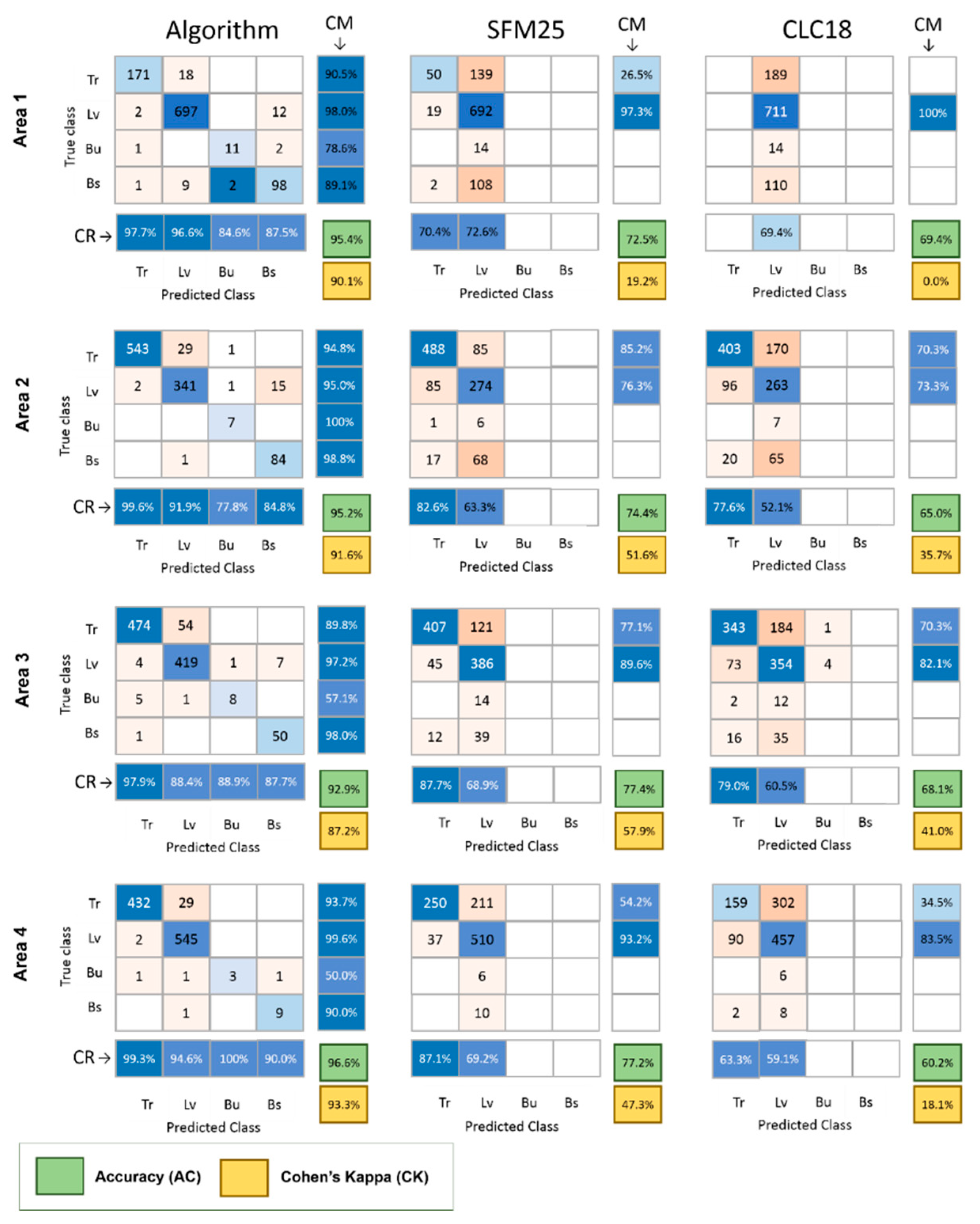
The results obtained with our algorithm showed high levels of performance based on the four different metrics (i.e., completeness, correctness, accuracy, and Cohen’s kappa) previously described (Figure 4). Our algorithm showed high values of accuracy (>92.8%) and Cohen’s kappa (>87.2%) for the four study areas. These metrics showed a lower performance for both SFM25 (<77.4% for AC and <57.9% for CK) and CLC18 (<69.4% for AC and <41.0% for CK). In relation to the areas defined as forest patches, at least 97.9% (CR) of the points were correctly classified. In addition, at least 89.8% (CM) of the points that were forests were detected. Detection and classification of the forest class showed the highest levels of performance among the four types of uses included in our study. The other types of land use also showed high levels of accuracy when using our own algorithm, especially the low vegetation class with values higher than 95.0% for completeness and 88.4% correctness. On the contrary, the two reference maps showed lower levels of accuracy for both completeness and correctness metrics (Figure 4). For CLC18, completeness of forest cover ranged from 0.0% to 70.3%, and correctness from 0.0% to 79.0%. These metrics showed higher levels of performance of SFM25 for the forest patches class: completeness 26.5–85.2% and correctness: 70.4–87.7%. Regarding the other vegetated class (shrublands and low vegetation), our algorithm also showed a better performance (correctness ranging from 88.4% to 96.6% and completeness from 95.0% to 99.6%) than the two reference maps (CLC18: 52.1–69.4% for correctness and 73.3–100% for completeness; SFM25 63.3–72.6% for correctness and 76.3–97.3% for completeness). The remaining two classes showed lower levels of performance for our algorithm (bare soil CM: 77.8–100% and CL 84.8–90.0%; and buildings CM: 50.0–100% and CL: 89.1–98.8%), but they were rarely identified by the two reference maps. As a consequence, validation metrics for those two classes were not calculated for CLC18 and SMF25.
4. Discussion
The algorithm developed in this study allows for the identification and delineation of different types of landscape features and land uses at the local level including forest/tree/woody vegetation patches of small size (<0.5 ha). This automatic method, based on the combination of point clouds derived from LiDAR data and aerial imagery, produces a higher spatial resolution output in comparison with other available datasets such as satellite imagery. The information used is freely available for the whole area of Spain, and every point within the point clouds contains spectral information in three bands (G, R and NIr) with different potential applications for classification of landscape patches by using vegetation indexes [10].
Spain is not the only country which has freely available LiDAR data of its whole territory. In recent years, a rising number of countries have conducted data collection for this kind of product. The increasing range of applications in different fields and the reduction of acquisition costs appear to be the main factors which have contributed to this rise. Moreover, some countries are investing efforts not only in the acquisition of data for their whole area but also in its periodic update [18,20,21,22,23,24,25,26,27,28]. Therefore, there is an increasing body of LiDAR datasets which will allow the use of the developed algorithm in many areas worldwide. In countries where the data are updated periodically, the algorithm can also be used for analysis of landscape dynamics and changes.
The spectral data from the aerial photographs used for the analysis were acquired by a non-calibrated digital camera that captures near infrared and visible wavelengths. These kinds of consumer-grade digital cameras are now established as a cost-effective method of monitoring plant health and phenology [38]. The combined use of infrared and visible observations provides more information than the use of just visible bands due to the strong contrast between infrared and visible reflection of vegetation, the high correlation of the three visible bands, and the possibilities of using spectral indices such as the NDVI. However, rigorous radiometric corrections are not applicable for images that have been processed and optimised for image visualization. In these cases, the pixel value may not represent the originally measured reflected brightness values and, therefore, it would not be possible to calculate the reflectance.
Our algorithm provided good results for identifying and delineating forest and woody patches (performance evaluated by confusion matrices and correctness and completeness values). In addition to this, our algorithm identified a higher level of vegetation cover than the other two alternative datasets compared (i.e., CLC18 and SFM25). Some of the differences, most of which related to the “low vegetation areas”, may be derived from areas of crops with temporal cover (arable areas) and showed positive NDVI values. This was when the aerial images were taken when the areas were covered by annual crops. Our methodology, despite having different and relevant strengths, is limited by the availability of adequate LiDAR and imagery information. Another shortcoming of our method is that it cannot establish the differences among forest types in terms of species composition, because this type of analysis demands the use of additional spectral data [55]. In addition, regarding the aboveground elevation, our method involves the generation of accurate terrain models from aerial point clouds. The generation of this type of model is not easy and has previously been tackled from many different perspectives [6]. The selection of the best terrain modelling algorithm remains subjective, however, as no single algorithm is objectively more accurate in all possible scenarios [56].
Finally, there are additional available sources of data that could be useful for similar aims to those assessed in this study. The European Union’s Earth Observation Programme “Copernicus” provides meaningful data. Copernicus supplies information with intermediate spatial resolution (pixel sizes between 20 and 100 m) which is periodically updated and includes relevant descriptors such as tree cover density or dominant leaf type [57]. Comparison between our algorithm and Copernicus-derived information was not included in this study, because Copernicus does not provide information about other woody elements (i.e., shrubs), bare soil areas, etc. In addition, the spatial resolution of the products derived from Copernicus can be limiting for delineating small forest patches, such as lineal woody elements, that are often narrower than 10 m [35]. In addition, additional applications can be derived from our methodology. For example, the digital model with the height above ground of the different vegetation covers can be used for multiple aims related to forest and land planning (e.g., estimation of biomass stocks [58] or fuel modelling for studies related to fire behaviour [59,60].
5. Conclusions
This study presented an automatic and easily reproducible algorithm for the classification and mapping of landscape patches with high spatial resolution (an approximately 2 m pixel size). The methodology developed combined information from LiDAR digital elevation models (for calculating the height of the different vegetation and artificial elements) and spectral information for G, R, and NIr bands derived from aerial imagery (for identifying the occurrence of vegetation covers). An important aspect of the proposed methodology was that we only used information available in public repositories.
The algorithm was tested on four different highly heterogeneous and highly fragmented areas in NW Spain, showing higher levels of accuracy than the two reference maps used as comparisons. The methodology presented here can constitute the basis for future high-detailed assessments at the landscape level of ecosystem dynamics and land cover changes. The method is easily reproducible, and for a 4 km2 area, the application only required seconds of data processing on a standard computer. The outputs generated were small-sized files (approximately 4 MB) which can allow the characterisation of larger study areas.
Author Contributions
Conceptualisation: J.V.R.-D. and C.C.; methodology: J.V.R.-D. and C.C.; formal analysis: J.V.R.-D., C.C. and C.P.; writing: J.V.R.-D., C.C., C.P., C.O. and C.S. All authors have read and agreed to the published version of the manuscript.
Funding
J.V.R.-D. obtained funding for this research from the Government of Asturias (Grant “Clarín” ACA17-02) under the FP7-Marie Curie-COFUND program of the European Commission. C.C. and C.S. received funding from the UK Natural Environment Research Council (NE/T001194/1).
Conflicts of Interest
The authors declare no conflict of interest. The funders had no role in the design of the study; in the collection, analyses, or interpretation of data; in the writing of the manuscript, or in the decision to publish the results.
References
- Vogt, P.; Riitters, K.H.; Iwanowski, M.; Estreguil, C.; Kozak, J.; Soille, P. Mapping landscape corridors. Ecol. Indic. 2007, 7, 481–488. [Google Scholar] [CrossRef]
- Buján, S.; González-Ferreiro, E.; Barreiro-Fernández, L.; Santé, I.; Corbelle, E.; Miranda, D. Classification of rural landscapes from low-density lidar data: Is it theoretically possible? Int. J. Remote Sens. 2013, 34, 5666–5689. [Google Scholar] [CrossRef]
- Hogg, O.T.; Huvenne, V.A.; Griffiths, H.J.; Linse, K. On the ecological relevance of landscape mapping and its application in the spatial planning of very large marine protected areas. Sci. Total Environ. 2018, 626, 384–398. [Google Scholar] [CrossRef] [PubMed]
- St-Onge, B.A.; Cavayas, F. Automated forest structure mapping from high resolution imagery based on directional semivariogram estimates. Remote Sens. Environ. 1997, 61, 82–95. [Google Scholar] [CrossRef]
- Asner, G.P.; Mascaro, J.; Muller-Landau, H.C.; Vieilledent, G.; Vaudry, R.; Rasamoelina, M.; Hall, J.S.; Van Breugel, M. A universal airborne LiDAR approach for tropical forest carbon mapping. Oecologia 2012, 168, 1147–1160. [Google Scholar] [CrossRef]
- Barreiro-Fernández, L.; Buján, S.; Miranda, D.; Diéguez-Aranda, U.; González-Ferreiro, E. Accuracy assessment of LiDAR-derived digital elevation models in a rural landscape with complex terrain. J. Appl. Remote Sens. 2016, 10, 016014. [Google Scholar] [CrossRef]
- Angelidis, I.; Levin, G.; Díaz-Varela, R.A.; Malinowski, R. Assessment of changes in formations of non-forest woody vegetation in southern Denmark based on airborne LiDAR. Environ. Monit. Assess. 2017, 189, 437. [Google Scholar] [CrossRef]
- Shao, G.; Wu, J. On the accuracy of landscape pattern analysis using remote sensing data. Landsc. Ecol. 2008, 23, 505–511. [Google Scholar] [CrossRef]
- Lechner, A.M.; Rhodes, J.R. Recent progress on spatial and thematic resolution in landscape ecology. Curr. Landsc. Ecol. Rep. 2016, 1, 98–105. [Google Scholar] [CrossRef] [Green Version]
- Jones, H.G.; Vaughan, R.A. Remote Sensing of Vegetation: Principles, Techniques, and Applications; Oxford University Press: Oxford, UK, 2010. [Google Scholar]
- Yang, C.; Westbrook, J.; Suh, C.; Martin, D.; Hoffmann, W.; Lan, Y.; Fritz, B.; Goolsby, J. An airborne multispectral imaging system based on two consumer-grade cameras for agricultural remote sensing. Remote Sens. 2014, 6, 5257–5278. [Google Scholar] [CrossRef] [Green Version]
- Navarro, L.M.; Pereira, H.M. Rewilding abandoned landscapes in Europe. In Rewilding European Landscapes; Springer: Berlin/Heidelberg, Germany, 2015; pp. 3–23. [Google Scholar]
- Forman, R.T.T.; Baudry, J. Hedgerows and hedgerow networks in landscape ecology. Environ. Manag. 1984, 8, 495–510. [Google Scholar] [CrossRef]
- Burel, F.; Baudry, J. Structural dynamic of a hedgerow network landscape in Brittany France. Landsc. Ecol. 1990, 4, 197–210. [Google Scholar] [CrossRef]
- Davies, Z.G.; Pullin, A.S. Are hedgerows effective corridors between fragments of woodland habitat? An evidence-based approach. Landsc. Ecol. 2007, 22, 333–351. [Google Scholar] [CrossRef]
- Jacqueminet, C.; Kermadi, S.; Michel, K.; Béal, D.; Gagnage, M.; Branger, F.; Jankowfsky, S.; Braud, I. Land cover mapping using aerial and VHR satellite images for distributed hydrological modelling of periurban catchments: Application to the Yzeron catchment (Lyon, France). J. Hydrol. 2013, 485, 68–83. [Google Scholar] [CrossRef]
- Kay, S.; Crous-Duran, J.; de Jalón, S.G.; Graves, A.; Palma, J.H.; Roces-Díaz, J.V.; Szerencsits, E.; Weibel, R.; Herzog, F. Landscape-scale modelling of agroforestry ecosystems services in Swiss orchards: A methodological approach. Landsc. Ecol. 2018, 33, 1633–1644. [Google Scholar] [CrossRef] [Green Version]
- Laurin, G.V.; Puletti, N.; Hawthorne, W.; Liesenberg, V.; Corona, P.; Papale, D.; Chen, Q.; Valentini, R. Discrimination of tropical forest types, dominant species, and mapping of functional guilds by hyperspectral and simulated multispectral Sentinel-2 data. Remote Sens. Environ. 2016, 176, 163–176. [Google Scholar] [CrossRef] [Green Version]
- Zhang, C.; Xie, Z.; Selch, D. Fusing lidar and digital aerial photography for object-based forest mapping in the Florida Everglades. GIScience Remote Sens. 2013, 50, 562–573. [Google Scholar] [CrossRef]
- PNOA, Plan Nacional Ortofotografia Aerea. Ministerio de Fomento. Gobierno de España. 2019. Available online: https://pnoa.ign.es/ (accessed on 2 November 2019).
- NLS, National Land Survey of Finland. Laser Scanning Data. 2019. Available online: https://www.maanmittauslaitos.fi/en/maps-and-spatial-data/expert-users/product-descriptions/laser-scanning-data (accessed on 2 November 2019).
- SDFE, Styrelsen for Datafrsyning og Effektivisering. 2019. Available online: https://sdfe.dk/data-skaber-vaerdi/nyheder/nyhedsarkiv/2019/apr/vigtige-hoejdedata-er-blevet-opdateret/ (accessed on 2 November 2019).
- GUGiK. Head Office of Geodesy and Cartography. ALS Point Cloud. 2019. Available online: https://eurogeographics.org/member/glowny-urzad-geodezji-i-kartografii/ (accessed on 2 November 2019).
- USGS, United States Geological Survey. LiDAR Data. 2019. Available online: https://www.usgs.gov/core-science-systems/ngp/3dep (accessed on 2 November 2019).
- Canadian GIS Canadian, LiDAR Data. 2019. Available online: https://canadiangis.com/free-canada-lidar-data.php (accessed on 2 November 2019).
- LINZ, Land Information New Zealand. LiDAR Data. 2019. Available online: https://data.linz.govt.nz/set/4702-nz-aerial-imagery/ (accessed on 2 November 2019).
- De Almeida, D.R.A.; Nelson, B.W.; Schietti, J.; Gorgens, E.B.; Resende, A.F.; Stark, S.C.; Valbuena, R. Contrasting fire damage and fire susceptibility between seasonally flooded forest and upland forest in the Central Amazon using portable profiling LiDAR. Remote Sens. Environ. 2016, 184, 153–160. [Google Scholar] [CrossRef]
- Hofton, M.; Blair, J.; Rabine, D.; Brooks, C.; Cornejo, H. Canopy height and structure measurements of Gabon from medium-footprint waveform lidar. In Proceedings of the 2017 IEEE International Geoscience and Remote Sensing Symposium (IGARSS), Fort Worth, TX, USA, 23–28 July 2017; IEEE: Piscataway, NJ, USA, 2017; pp. 4294–4295. [Google Scholar]
- Hopkinson, C.; Chasmer, L.; Gynan, C.; Mahoney, C.; Sitar, M. Multisensor and multispectral lidar characterization and classification of a forest environment. Can. J. Remote Sens. 2016, 42, 501–520. [Google Scholar] [CrossRef]
- Stal, C.; Briese, C.; De Maeyer, P.; Dorninger, P.; Nuttens, T.; Pfeifer, N.; De Wulf, A. Classification of airborne laser scanning point clouds based on binomial logistic regression analysis. Int. J. Remote Sens. 2014, 35, 3219–3236. [Google Scholar] [CrossRef] [Green Version]
- Habib, A.F.; Chang, Y.C.; Lee, D.C. Occlusion-based methodology for the classification of LiDAR data. Photogram. Eng. Remote Sens. 2009, 75, 703–712. [Google Scholar] [CrossRef]
- Ao, Z.; Su, Y.; Li, W.; Guo, Q.; Zhang, J. One-class classification of airborne LiDAR data in urban areas using a presence and background learning algorithm. Remote Sens. 2017, 9, 1001. [Google Scholar] [CrossRef] [Green Version]
- Zhao, X.; Guo, Q.; Su, Y.; Xue, B. Improved progressive TIN densification filtering algorithm for airborne LiDAR data in forested areas. ISPRS J. Photogram. Remote Sens. 2016, 117, 79–91. [Google Scholar] [CrossRef] [Green Version]
- Badenko, V.; Zotov, D.; Muromtseva, N.; Volkova, Y.; Chernov, P. Comparison of Software for Airborne Laser Scanning Data Processing in Smart City Applications. Int. Arch. Photogram. Remote Sens. Spat. Inform. Sci. 2019, XLII-5/W2. [Google Scholar] [CrossRef] [Green Version]
- Díaz-Varela, E.; Roces-Díaz, J.V.; Álvarez-Álvarez, P. Detection of landscape heterogeneity at multiple scales: Use of the Quadratic Entropy Index. Landsc. Urban Plan. 2016, 153, 149–159. [Google Scholar] [CrossRef]
- ASPRS, The American Society for Photogrammetry & Remote Sensing. LAS Specification 1.4. 2019. Available online: http://www.asprs.org/wp-content/uploads/2019/07/LAS_1_4_r15.pdf (accessed on 10 February 2020).
- Hexagon Systems. Leica Geosystems. Leica RCD30 Medium Format RGBN Camera. 2020. Available online: https://leica-geosystems.com/es-es/products/airborne-systems/imaging-sensors/leica-rcd30 (accessed on 25 January 2020).
- Pettorelli, N.; Vik, J.O.; Mysterud, A.; Gaillard, J.-M.; Tucker, C.J.; Stenseth, N.C. Using the satellite-derived NDVI to assess ecological responses to environmental change. Trends Ecol. Evol. 2005, 20, 503–510. [Google Scholar] [CrossRef]
- Rouse Jr, J.; Haas, R.H.; Schell, J.A.; Deering, D.W. Monitoring vegetation systems in the Great Plains with ERTS. 1974. Available online: https://ntrs.nasa.gov/search.jsp?R=19740022614 (accessed on 9 February 2020).
- Welles, J.M. Some indirect methods of estimating canopy structure. Remote Sens. Rev. 1990, 5, 31–43. [Google Scholar] [CrossRef]
- Xu, D.; Guo, X.; Li, Z.; Yang, X.; Yin, H. Measuring the dead component of mixed grassland with Landsat imagery. Remote Sens. Environ. 2014, 142, 33–43. [Google Scholar] [CrossRef]
- Berra, E.F.; Gaulton, R.; Barr, S. Commercial off-the-shelf digital cameras on unmanned aerial vehicles for multitemporal monitoring of vegetation reflectance and NDVI. IEEE Trans. Geosci. Remote Sens. 2017, 55, 4878–4886. [Google Scholar] [CrossRef] [Green Version]
- Verhoeven, G.J.; Smet, P.F.; Poelman, D.; Vermeulen, F. Spectral characterization of a digital still camera’s NIR modification to enhance archaeological observation. IEEE Trans. Geosci. Remote Sens. 2009, 47, 3456–3468. [Google Scholar] [CrossRef]
- Nijland, W.; De Jong, R.; De Jong, S.M.; Wulder, M.A.; Bater, C.W.; Coops, N.C. Monitoring plant condition and phenology using infrared sensitive consumer grade digital cameras. Agric. For. Meteorol. 2014, 184, 98–106. [Google Scholar] [CrossRef] [Green Version]
- Zhang, W.; Qi, J.; Wan, P.; Wang, H.; Xie, D.; Wang, X.; Yan, G. An easy-to-use airborne LiDAR data filtering method based on cloth simulation. Remote Sens. 2016, 8, 501. [Google Scholar] [CrossRef]
- EEA, European Environment Agency. CORINE Land Cover. 2019. Available online: https://land.copernicus.eu/pan-european/corine-land-cover/clc2018 (accessed on 30 October 2019).
- MAPA, Ministerio de Agricultura, Pesca y Alimentacion. Mapa Foresta de España 1:25000. 2018. Available online: https://www.mapa.gob.es/es/desarrollo-rural/temas/politica-forestal/inventario-cartografia/mapa-forestal-espana/mfe_25.aspx (accessed on 30 October 2019).
- Roces-Díaz, J.V.; Burkhard, B.; Kruse, M.; Müller, F.; Díaz-Varela, E.R.; Álvarez-Álvarez, P. Use of ecosystem information derived from forest thematic maps for spatial analysis of ecosystem services in northwestern Spain. Landsc. Ecol. Eng. 2017, 13, 45–57. [Google Scholar] [CrossRef]
- Campos, P.; Caparrós, A.; Oviedo, J.L.; Ovando, P.; Álvarez-Farizo, B.; Díaz-Balteiro, L.; Carranza, J.; Beguería, S.; Díaz, M.; Herruzo, A.C. Bridging the Gap Between National and Ecosystem Accounting Application in Andalusian Forests, Spain. Ecol. Econ. 2019, 157, 218–236. [Google Scholar] [CrossRef]
- Hengl, T. Finding the right pixel size. Comput. Geosci. 2006, 32, 1283–1298. [Google Scholar] [CrossRef]
- Richards, J.A.; Jia, X. Remote Sensing Digital Image Analysis, 4th ed.; Springer: Berlin/Heidelberg, Germany, 2006; p. 454. [Google Scholar]
- Cohen, J. A coefficient of agreement for nominal scales. Educ. Psychol. Meas. 1960, 20, 37–46. [Google Scholar] [CrossRef]
- Tallón-Ballesteros, A.J.; Riquelme, J.C. Data mining methods applied to a digital forensics task for supervised machine learning. In Computational Intelligence in Digital Forensics: Forensic Investigation and Applications; Muda, A., Choo, Y.H., Abraham, A., Srihari, S.N., Eds.; Springer: Berlin/Heidelberg, Germany, 2014; Volume 555, pp. 413–428. [Google Scholar]
- Pontius Jr, R.G.; Millones, M. Death to Kappa: Birth of quantity disagreement and allocation disagreement for accuracy assessment. Int. J. Rem. Sens. 2011, 32, 4407–4429. [Google Scholar] [CrossRef]
- Cho, M.A.; Mathieu, R.; Asner, G.P.; Naidoo, L.; van Aardt, J.; Ramoelo, A.; Debba, P.; Wessels, K.; Main, R.; Smit, I.P. Mapping tree species composition in South African savannas using an integrated airborne spectral and LiDAR system. Remote Sens. Environ. 2012, 125, 214–226. [Google Scholar] [CrossRef]
- Buján, S. La tecnología LiDAR al servicio de la representación del relieve y la identificación de coberturas del suelo. Ph.D. Thesis, Universidade de Santiago de Compostela, Lugo, Spain, 2019. [Google Scholar]
- EEA, European Environment Agency. High Resolution Layers. 2019. Available online: https://land.copernicus.eu/pan-european/high-resolution-layers/forests (accessed on 30 October 2019).
- Novo-Fernández, A.; Barrio-Anta, M.; Recondo, C.; Cámara-Obregón, A.; López-Sánchez, C.A. Integration of National Forest Inventory and Nationwide Airborne Laser Scanning Data to Improve Forest Yield Predictions in North-Western Spain. Remote Sens. 2019, 11, 1693. [Google Scholar] [CrossRef] [Green Version]
- González-Olabarria, J.-R.; Rodríguez, F.; Fernández-Landa, A.; Mola-Yudego, B. Mapping fire risk in the Model Forest of Urbión (Spain) based on airborne LiDAR measurements. For. Ecol. Manag. 2012, 282, 149–156. [Google Scholar] [CrossRef]
- Sánchez Sánchez, Y.; Martínez-Graña, A.; Santos Francés, F.; Mateos Picado, M. Mapping wildfire ignition probability using sentinel 2 and LiDAR (Jerte Valley, Caceres, Spain). Sensors 2018, 18, 826. [Google Scholar] [CrossRef] [PubMed] [Green Version]
Figure 1.
Location of the four 2 × 2 km study areas used in this analysis. Specific details about the coordinates of their upper-left corners (ETRS89/WGS84: Longitude, Latitude) are Area 1: −8.9264°, 42.9738°; Area 2: −8.1604°, 43.3858°; Area 3: −8.1577°, 43.5838°; Area 4: −7.6178°, 43.3625°.
Figure 1.
Location of the four 2 × 2 km study areas used in this analysis. Specific details about the coordinates of their upper-left corners (ETRS89/WGS84: Longitude, Latitude) are Area 1: −8.9264°, 42.9738°; Area 2: −8.1604°, 43.3858°; Area 3: −8.1577°, 43.5838°; Area 4: −7.6178°, 43.3625°.

Figure 2.
Workflow of the main stages of the proposed method on a 2 x 2 km tile from PNOA (National Air Orthophotography Programme in Spain).
Figure 2.
Workflow of the main stages of the proposed method on a 2 x 2 km tile from PNOA (National Air Orthophotography Programme in Spain).

Figure 3.
False colour RGB representation from aerial imagery and land use classification (algorithm developed for this study, SFM25, and CLC18) for the four study areas.
Figure 3.
False colour RGB representation from aerial imagery and land use classification (algorithm developed for this study, SFM25, and CLC18) for the four study areas.

Figure 4.
Confusion matrix, accuracy (AC), Cohen’s kappa coefficient (CK), completeness (CM), and correctness (CR) obtained with the proposed algorithm. True classes were determined by visual inspection and from SFM25 and CLC18 maps. Abbreviations: Tr: forest and trees, Lv: shrublands and low vegetation, Bs: bare soil, Bu: buildings. Validation metrics: CM: completeness. CR: correctness.


Table 1.
Descriptions of the four types of land uses used for our developed algorithm and for the two reference maps used for validation: Corine Land Cover 2018 (CLC18) [46] and Spanish Forest Map 1:25,000 (MFE25) [47]. In the third column, the numbers in brackets show the code from CLC18 classification.
| Class | Algorithm | CLC18 (Corine Land Cover 2018) Classes Included | SFM25 (Spanish Forest Map 1:25,000) Classes Included |
|---|---|---|---|
| Forest and trees | High (i.e., above the elevation threshold) and vegetated (i.e., the normalised difference vegetation index NDVI threshold) | Forests (31) | Polygons where tree cover was >50% (or where tree cover > shrub/grass cover) |
| Shrub and low vegetation | Low (i.e., below the elevation threshold) and Vegetated | Artificial vegetated areas (14) Permanent crops (22) Pastures (23) Heterogeneous agricultural areas (24) Shrub and/or herbaceous vegetation (32) | Areas where shrub/grass cover was >50% |
| Buildings and artificial areas | High (i.e., above the elevation threshold) and non-vegetated (i.e., below the NDVI threshold) | Urban fabrics (11) Industrial areas (12) | No applicable (this type of cover was not included in this dataset) |
| Bare soil | Low (i.e., below the elevation threshold) and non-vegetated (i.e., below the NDVI threshold) | Arable lands (21) Mines and construction sites (13) Open spaces with little vegetation (33) | Areas without vegetation cover |
© 2020 by the authors. Licensee MDPI, Basel, Switzerland. This article is an open access article distributed under the terms and conditions of the Creative Commons Attribution (CC BY) license (http://creativecommons.org/licenses/by/4.0/).
Share and Cite
MDPI and ACS Style
Roces-Díaz, J.V.; Cabo, C.; Prendes, C.; Ordoñez, C.; Santín, C. Automatic Delineation of Forest Patches in Highly Fragmented Landscapes Using Coloured Point Clouds. Forests 2020, 11, 198. https://doi.org/10.3390/f11020198
AMA Style
Roces-Díaz JV, Cabo C, Prendes C, Ordoñez C, Santín C. Automatic Delineation of Forest Patches in Highly Fragmented Landscapes Using Coloured Point Clouds. Forests. 2020; 11(2):198. https://doi.org/10.3390/f11020198
Chicago/Turabian StyleRoces-Díaz, José V., Carlos Cabo, Covadonga Prendes, Celestino Ordoñez, and Cristina Santín. 2020. "Automatic Delineation of Forest Patches in Highly Fragmented Landscapes Using Coloured Point Clouds" Forests 11, no. 2: 198. https://doi.org/10.3390/f11020198
Note that from the first issue of 2016, this journal uses article numbers instead of page numbers. See further details here.