The SOS Platform: Designing, Tuning and Statistically Benchmarking Optimisation Algorithms


1
Institute of Artificial Intelligence, School of Computer Science and Informatics, De Montfort University, Leicester LE1 9BH, UK
2
Department of Information Engineering and Computer Science, University of Trento, 38123 Trento, Italy
*
Author to whom correspondence should be addressed.
Mathematics 2020, 8(5), 785; https://doi.org/10.3390/math8050785
Submission received: 31 March 2020
/
Revised: 24 April 2020
/
Accepted: 5 May 2020
/
Published: 13 May 2020
(This article belongs to the Special Issue Evolutionary Computation & Swarm Intelligence)
Abstract
:We present Stochastic Optimisation Software (SOS), a Java platform facilitating the algorithmic design process and the evaluation of metaheuristic optimisation algorithms. SOS reduces the burden of coding miscellaneous methods for dealing with several bothersome and time-demanding tasks such as parameter tuning, implementation of comparison algorithms and testbed problems, collecting and processing data to display results, measuring algorithmic overhead, etc. SOS provides numerous off-the-shelf methods including: (1) customised implementations of statistical tests, such as the Wilcoxon rank-sum test and the Holm–Bonferroni procedure, for comparing the performances of optimisation algorithms and automatically generating result tables in PDF and LATEX formats; (2) the implementation of an original advanced statistical routine for accurately comparing couples of stochastic optimisation algorithms; (3) the implementation of a novel testbed suite for continuous optimisation, derived from the IEEE CEC 2014 benchmark, allowing for controlled activation of the rotation on each testbed function. Moreover, we briefly comment on the current state of the literature in stochastic optimisation and highlight similarities shared by modern metaheuristics inspired by nature. We argue that the vast majority of these algorithms are simply a reformulation of the same methods and that metaheuristics for optimisation should be simply treated as stochastic processes with less emphasis on the inspiring metaphor behind them.
1. Introduction
Experimentalism plays a major role in all fields of metaheuristic optimisation, such as evolutionary computation (EC) and swarm intelligence (SI). It can be a time-demanding, repetitive and tedious process to fine-tune optimisers, compare them or validate new algorithmic strategies on benchmark problems. Due to their stochastic nature, and the lack of theoretical knowledge on the internal dynamics of many of these nature-inspired approaches, their algorithmic design is partially blind and often empirically performed through a series of trial-and-error phases [1]. This involves using several artificially built benchmark problems simulating characteristics present in real-world scenarios, but for which some knowledge is available. The use of such testbed problems is preferable since they usually have a more reasonable execution time than real-world applications, they can be run on any machine, this being e.g., a modest personal computer or a high-performance computing system, and they are not subject to time and other limitations typical of real-world scenarios, unless these are purposely imposed to reproduce a specific situation. Thus, these problems are suitable choices for performing the algorithmic design phase of novel algorithms and evaluating the performances of specific operators and algorithmic variants. By design, these problems display particular characteristics reported in the corresponding technical reports in term of, e.g., ill-conditioning, separability, m-separability, noise, modality (i.e., multimodal or unimodal function), etc., allowing also for studying the algorithmic behaviour of certain operators [2,3,4].
In this light, the research community benefits from platforms featuring a large number of algorithms and benchmark problems, such as the Decision Tree for Optimisation software [5], the COCO platform [6], IOHprofiler [7], jMetal [8] or PlatEMO [9]. However, the availability of code implementing complete benchmark suites and popular optimisation algorithms is only one amongst the many requirements an algorithm designer has to work efficiently and focus algorithmic issues rather than having to deal with the implementation of ancillary software. The other functionalities that a research-oriented platform for metaheuristic optimisation should have are:
- result visualisation methods (in both tabular and graphical formats).
On top of that, such a platform should provide:
- a vast and heterogeneous number of benchmark functions and real-world testbed problems;
- several state-of-the-art algorithms to be used for comparisons with newly-designed algorithms;
- libraries with implementations of the most popular algorithmic operators such as mutation methods, crossover methods, parent and survivor selection mechanisms, heuristics selection methods for memetic computing (MC) and hyperheuristic approaches, etc.;
- a system to spread the runs over multiple cores and threads, thus speeding up the data generation process, and automatically collecting and processing raw data into meaningful information.
Additionally, the platform should be based on:
- open source software, so that researchers can freely use it and build upon it;
- a simple and flexible structure so that new problems and algorithms can be easily added.
The Stochastic Optimisation Software, henceforth SOS, exhibits the aforementioned key features, thus facilitating the design, the evaluation and the use of metaheuristic optimisation algorithms. Thanks to its simple and extendible structure, SOS can be easily used by researchers to implement new algorithms and compare their performances with those of several other benchmark algorithms. The most recent SOS release, available in the Zenodo repository [17], contains over fifty ready-to-use algorithms amongst single-solution and population-based metaheuristics, as those described in [18], all belonging to established optimisation paradigms such as evolutionary algorithms (EA) [19], swarm intelligence (SI) optimisation [20] and other hybrid schemes. Hence, it provides users with a variety of techniques to explore multiple flavours of metaheuristic/stochastic optimisation. More algorithms will be added in future releases. Researchers can benefit in several ways from having such a large availability of algorithms. Firstly, this means that comparison algorithms do not need to be implemented as they are already present and ready to be executed. Secondly, their source code is accessible and can be modified to create new variants or simply visioned as a source of inspiration for implementing other algorithms or algorithmic operators. Thirdly, they can combine the existing algorithms or embed them into new algorithms, thus creating novel hybrid methods as done, e.g., in memetic computing and hyperheuristics [3,21,22,23,24]. It must be highlighted that implementing algorithms in SOS is quite simple since most algorithmic operators are provided by the platform. Moreover, the “template” class Algorithm, which is equipped with several ancillary methods, can simply be extended to implement any metaheuristic, regardless of the optimisation family. In this light, SOS also represents an excellent pedagogical tool for teaching purposes and can be used to give guidance to students while implementing optimisation algorithms. Indeed, since 2015 the “student” version of SOS has been used to teach the master module “Computational Intelligence Optimisation” led by Dr Fabio Caraffini at De Montfort University (Leicester, UK), for which it was originally designed before being extended to the current form. Researchers willing to collaborate and add code (algorithms, real-world problems, etc.) to the platform are welcome and invited to get in touch to be added to the SOS GitHub repository (whose link is provided in Table 1). Finally, it is worth mentioning that due to the simplicity in adding problems and algorithms, SOS represents a useful tool for practitioners who might have less interest in the algorithmic design but a high need for off-the-shelf implementations of optimisation algorithms. The remainder of this article is structured as follow:
- Section 2 presents the SOS software platform and provides detailed descriptions of its features;
- Section 3 focuses on benchmarking optimisation algorithms with SOS and lists the available benchmark suites, including established benchmarks and one customised benchmark;
- Section 4 first provides a literature review on statistical methods for comparing stochastic optimisation algorithms, then describes the implementation and working mechanisms of three statistical analyses available in SOS;
- Section 5 reports on the result visualisation capabilities of SOS and provides “how-to” examples based on studies from the current literature in metaheuristic optimisation;
- Section 6 summarises the key points of this article and remarks on the novel aspects of SOS;
- Appendix A gives additional details on the routine used to produce average fitness trend graphs.
2. The SOS Platform
For portability reasons, SOS is coded in Java, thus being platform-independent. To speed up the execution of extensive experiments, some benchmark suites are also available in the form of C/C++ native libraries (compiled for MS Windows, MAC OS and Linux machines) using the Java Native Interface (JNI). By default, SOS spreads the “runs” (i.e., the optimisation processes in which one algorithm optimises one problem) over the available threads and executes them in parallel. In order to avoid that, e.g., if the experiment is executed on a laptop or personal computer and CPU power must be saved of other applications, it is possible to switch to the single-thread mode by means of the setter method setMT(boolean MT) of the class Experiment (i.e., its Boolean flag variable must be set to false). By looking at the code available in [17], one can notice that in the current release, a strong emphasis is given to real-valued box-constrained single-objective optimisation, also known as “single-objective continuous optimisation” in the EC community. Nevertheless, SOS can be used for addressing other optimisation domains such as discrete or combinatorial ones.
2.1. Functional Overview
SOS is research-oriented and is designed to have an intuitive structure making it straightforward to use for both expert algorithm designers in the research community and, most importantly, for practitioners and students from different subject fields. Indeed, to execute an experiment, it is sufficient to add a class, which extends the abstract Experiment class, in the homonym folder (package). Such a class will automatically inherit the add methods, which can be used to add algorithms and problems to the experiment, and other methods to set, e.g., the allowed computational budget (if not set, by default, this is assumed to be equal to with n being the dimensionality of the problem) and the number of runs to be performed. Subsequently, a main method must be written to launch one or multiple experiments. To do this, the methods of the utility class RunAndStore can be imported to, e.g.,:
- execute a list of experiments having different budgets, number of runs, problems and algorithms, or the same experiments repeated for different dimensionalities (if the problems are scalable);
- generate log files describing the performed experiments (i.e., the list of problems and their corresponding details, e.g., dimensionality, as well as the parameter setting, number of runs, etc.);
- store raw data and process them into results tables and plottable formats, as shown in Section 5.
It must be said that the computational budget can be arbitrarily allocated for each experiment using the provided setter methods (described in the SOS documentation). These can be used to either set a multiplicative factor (which multiplies n, thus adjusting the budget of each function in the experiment based on its dimensionality) or set a fixed amount of functional calls. This poses limitations on the maximum number of allowed functional evaluations, but does not prevent the algorithms from stopping the search earlier. Indeed, each algorithm can be equipped with a customised “stop” criterion based, e.g., on the number of improvements on the fitness values, the use of thresholds specifying a desired fitness tolerance, an incremental improvement value, etc.
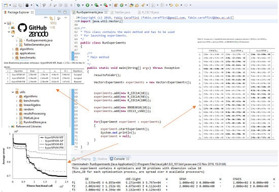
Figure 1 shows an example of a main method used for executing a list of experiments and displaying the final outputs, i.e., tables and graphs, generated by SOS after processing the results. With reference to the latest release in [17], a large number of experiment files can be found in the experiments package, while several examples of main files (showing different configurations and options for storing and processing results in different formats) are available in the mains package. Among these examples, the most convenient one to be used as a template is the class RunExperiments, shown in Figure 1, which is located in the default package of the SOS platform. More indications on how to write an experiment class are given in Section 2.2 and graphically shown in Figure 2.
To minimise the need for referring to a detailed document, SOS is equipped with a high number of self-explanatory example classes. Moreover, the clear nomenclature used for methods, variable types and class names and the user-friendly structure of the proposed platform give guidance to the users, who may not even need further indications. Nonetheless, the software documentation is available online to provide users with further information on SOS packages, classes and methods. Table 1 displays relevant links to SOS web pages, from which SOS documentation can be accessed. These web pages are kept up-to-date, and the documentation itself is constantly updated to reflect any major changes of the platform. This documentation plays a key role for those who intend to modify SOS source code, extend it or customise it to a specific need.
SOS makes it very easy to add new algorithms and new problems that are fully compatible with the platform, so as to exploit its full capabilities. For the sake of good organisation, it is suggested to place their implementation into the three provided packages: algorithms, benchmarks and applications.
The algorithms folder currently contains a vast list of optimisation algorithms for continuous optimisation, which, in may cases, can be run under different combinations of variation and/or selection operators, thus providing an even higher number of choices. This results in a good balance between established optimisation methods, such as differential evolution (DE) [1,25], simulated annealing (SA) [26], genetic algorithms (GAs), particle swarm optimisation (PSO) [27] and evolution strategies (ES) [28,29,30], and more modern optimisers such as single particle optimisation [31], self-adaptive algorithms [32,33,34,35,36,37,38] and MC/hyperheuristic approaches [3,23,24,39,40,41]. For a complete list, one can refer to the algorithms folder from [17] or check the online documentation. More information on the SOS algorithms is given in Section 2.3.
The benchmarks folder contains the implementation of problems taken from some established benchmark suites for optimisation. SOS implements several testbed problems and complete benchmarks suites that can be added in the experiment files. A complete list of these optimisation problems and their relevant documentation is provided in Section 3. Furthermore, a novel benchmark suite is presented in Section 3.
The applications folder is where specific real-world applications should be implemented. Some examples from the literature, e.g., the code for the application described in [23], and from a benchmark suite for real-world problems [42] are available in this folder.
Following the execution of an experiment, the produced raw data can be processed by means of the classes in the package utils.resultsProcessing. These provide several functionalities, including:
- the execution of statistical tests for comparing optimisation algorithms, described in Section 4, including the advanced statistical analysis (ASA) presented in Section 4.3;
- the generation of plottable files suitable for Tikz, Matplotlib, Gnuplot or MATLAB scripts for displaying best/median/worse/average fitness trends, as shown in Section 5 and Appendix A;
- the generation of
![Mathematics 08 00785 i001]() tables (both source code and PDF files are produced) showing results in terms the average fitness value (or average error w.r.t. the known optimum, if available) with the corresponding standard deviation and further statistical evidence, as explained in Section 4 and graphically shown in Section 5.
tables (both source code and PDF files are produced) showing results in terms the average fitness value (or average error w.r.t. the known optimum, if available) with the corresponding standard deviation and further statistical evidence, as explained in Section 4 and graphically shown in Section 5.
The file TabGen.java, located in the Mains folder, contains the methods for generating the previously mentioned tables and graphical outputs and can be modified to customise the production of tables with different layouts and informative content, as discussed in Section 5.
It is worth stressing the fact that having a fast way to visualise results in multiple formats is a key element to facilitate research in the area of stochastic optimisation. This feature is indeed very useful since the raw data are automatically processed and the ![Mathematics 08 00785 i001]() source of the comparative tables is generated without any user intervention, together with the corresponding PDF files.
source of the comparative tables is generated without any user intervention, together with the corresponding PDF files.
 source of the comparative tables is generated without any user intervention, together with the corresponding PDF files.
Moreover, this also accelerates the algorithmic design phase, which is often performed empirically through several trial-and-error steps. At each step, different variants of the same algorithm must be compared and tables must be generated. This is quite common in the EC filed where using a different combination of variation operators [19] with different combinations of parents and survivors selection schemes [19] can lead to a variety of possible algorithmic behaviours. The same issue arises when designing MC and hyperheuristic algorithms, for which several coordination schemes must be tested to ensure high performances [3,21,22,24]. This aspect suggests that the empirical design approach can only produce algorithms tailored to the problem(s) considered during the design phase. To some extent, this issue can be considered analogous to the training process in machine learning.
In this light, the algorithmic design process is not so different from the process performed to choose the less disruptive correction method for handling infeasible solutions generated while addressing a problem [1,16,43] or from the fine-tuning process performed to find the most appropriate set of parameters for an algorithm A meant to address specific problem P.
2.2. Parameters’ Fine-Tuning
Metaheuristics for optimisation must be tuned on the problem at hand to make them achieve their full potential and return high-quality solutions. Against the original common belief that a “universal” algorithm could have been designed, theoretical achievements such as, first and foremost, the “no free lunch theorems” (NFLTs) for optimisation [47,48] highlighted the need for fine-tuning, self-adaptation and the use of problem-specific operators.
However, finding the optimal parameter configuration is an optimisation problem itself. Despite meta-optimisation strategies having been proposed [49,50], these do not completely solve the problem and are arguable, since they introduce further complexity due to the fact that also the meta-optimiser might need to be fine-tuned. Furthermore, the fact that most real-world optimisation problems are black-box systems, i.e., little or no analytical information on the fitness function is available, increases the difficulty in finding an exact method for finding the optimal configuration of parameters.
Under these circumstances, the parameters’ tuning process is necessarily performed empirically, thus resulting in a rather time-consuming and tiresome activity. SOS can be used to accelerate and facilitate this task significantly as: (1) the same algorithm can be included multiple times in the same experiment file with different parameter configurations; (2) runs can be spread over the available processors and threads to speed up the generation of results; (3) raw data are statistically analysed and results automatically displayed in compact, yet highly informative tables and graphs (see the examples provided in Section 5). Hence, the only portion of code that one needs to write to apply and tune an algorithm A on a specific real-world problem P with SOS is actually the code implementing P.
It must be pointed out that also artificially built testbed problems, as those already implemented in SOS (see Section 3), can play a role in the parameter tuning process. Indeed, studying how the algorithmic behaviour of a metaheuristic algorithm changes under different configurations of its parameters on these benchmarks can help shed light on how to perform the tuning process. By using testbed problems, whose mathematical properties (e.g., differentiability, separability, modality, ill-conditioning, etc.) are known, one can understand, e.g., the effect of the parameters in relation to these mathematical features. As a result, specific regions of the parameter space could be detected to obtain a robust general-purpose behaviour rather than a very problem-specific one, or to strengthen exploitation capabilities rather than exploration capabilities, or to minimise the rise of algorithmic structural biases, as done in [1,12,43], the generation of a high number of infeasible solutions, as done in [1,16], or premature convergence [51] and stagnation [52], as done in [11].
Most of the aforementioned studies have been performed with SOS, and their experiment files can be found in [17]. Portions of the code from three experiment files are reported in Figure 2, which helps understand how the parameter space of an algorithm can be explored in SOS.
In Figure 2a, four DE variants are added into an experiment named ExperimentDE by using the constructor super(probDim,5000,“ExperimentDE”). Therefore, all the produced text files containing raw data will be saved in a homonym folder, located inside the SOS default results folder. From the constructor method, it can be seen that a maximum computational budget of fitness functional calls, with n being the dimensionality of the problem, is used. Clearly, this experiment file contains scalable testbed problems and not real-world applications since the dimensionality of the problems is not fixed and passed as an argument with the variable probDim. The number of performed runs, 30 in this case, is specified with the command setNrRuns(30) (SOS performs 100 runs if not specified otherwise). It must be noted that all the other parameters, apart from the population size, are fixed. This means that this experiment will only study the effect of varying population sizes, which are in this case equal to the problem dimension as required for the studies in [4,53], which can be read for further details. To execute this experiment with increasing problem dimensionalities, and therefore, in turn, increasing population sizes, it is sufficient to instantiate objects with increasing probDim values by calling the class constructor in the file RunExperiments.java (as shown in the example of Figure 1). It is interesting to note that, to avoid confusion, a name is assigned to each DE variant (e.g., a.setID("DErn1bin")). The assigned name will show up in the generated tables. If a name is not provided, as in the example of Figure 2c, it will be automatically assigned equal to the class name of the algorithm. Therefore, in this case, the assigned names would start with DE, followed by “-i”, where “i” represents a counter incremented every time an algorithm is added to an experiment. In a nutshell, if names were not specified in the example of Figure 2a, tables would display DE-1, DE-2, DE-3 and DE-4, since all the algorithms in this experiment are instances of the DE class. Differently, in Figure 2b, the same DE variant, namely DE/rand/1/exp, is added four times to the experiment, with four different values for the so-called “crossover ratio” parameter . As can be seen at the bottom of the figure, all 30 rotated problems from the benchmark suite proposed in Section 3 are added to this experiment. Hence, its purpose is to understand the impact of the value on DE/rand/1/exp when facing different problems.
Finally, Figure 2c shows a very compact and fast way for configuring a large experiment in SOS, in which 12 DE variants are equipped with four different correction strategies for handling infeasible solutions, for a total of 48 different algorithms to tune. From the left-hand side of the figure, it can be seen that the DE variants are obtained by combining the six mutations with the two crossover operators in the DEMutations and CrossOvers arrays, respectively. The four correction strategies are in the corrections array. For details about the adopted notation for DE variants and correction strategies, one can consult the articles [1,12] and the results in [45]. For each algorithm, the explored parameters space is defined as the Cartesian product of the three sets represented by the populationSizes array, containing three population sizes, the FValues array, containing 10 equally spaced values for the so-called “scale factor” parameter F in the range , and the CRValues array, containing five equally spaced values for in the range . Hence, each one of the 48 algorithms is tuned over a set of 150 possible combinations of the three parameters. In total, this means that optimisation processes are executed, with being the number of runs performed for each problem added to this experiment. The full code for this example, named ExampleTuning, is located in the mains package. For demonstration purposes, is set equal to 10, and the computation budget is set to .
2.3. Adding New Algorithms and Problems
The literature is currently saturated with “novel” nature-inspired optimisation metaphors claiming to mimic collaborative or individual behaviours of animals [54,55,56,57,58,59,60,61], human activities [62,63,64] or other natural phenomena [65,66,67]. The contribution made by most of these new optimisation paradigms is arguable, as in general, they are very similar to more established EAs, such as GA, DE or ES, or swarm intelligence algorithms such as PSO. Furthermore, these new metaheuristics are by definition subject to the NFLTs, and as such, it can be shown that, unless they are highly fine-tuned, they cannot outperform classic algorithms over all possible problems. It must be remarked that also amongst the most established optimisation frameworks, some similarities can be detected in support of the thesis that taxonomies based on metaphors inspiring the algorithm design could (and should) be indeed avoided. To provide some examples, it is sufficient to observe that DE mutations, being linear combinations of individuals from the population [1,25], operate in the same way as the arithmetic crossover used in real-valued GAs and other EAs [19]. Similarly, it can be observed that the lack of parent selection in SI frameworks, such as in PSO [27], is simply moved in the perturbation operator, since this requires the definition of the neighbourhood of the candidate solution to be perturbed to find its local best solution.
In this light, a scientific approach to describe a metaheuristic for optimisation is by considering it as a stochastic process returning a near-optimal solution for an optimisation problem. Regardless of the metaphor behind them, all metaheuristic methods are the expression of the same concept and aim at reaching a good balance between exploration of the fitness landscape, looking for promising basins of attraction, and their exploitation, to refine the search and find local optimal solutions (i.e., maxima or minima according to the need). This dynamic process can alternate such phases as appropriate to keep looking for the global optimum, without prematurely converging to a locally optimal solution or stagnating without being able to return any satisfactory near-optimal solution.
Hence, it makes sense to analyse the algorithmic structure of modern nature-inspired optimisation algorithms and extrapolate a common, high level, general skeleton to use as a template for their implementation. This is done in SOS by means of the abstract class Algorithm, from which all algorithms inherit ancillary and auxiliary methods (e.g., for algorithm execution, storing the fitness trend, setting or generating the initial guess, etc.) and extend only the parts to be customised to implement the desired optimisation framework (e.g., GA, DE, a hybrid method or a completely new optimisation paradigm). Therefore, any class file extending Algorithm is already equipped with all the methods needed to add the algorithm to an experiment file and execute it as described in the previous section, while it must implement one method, named execute, which returns an object of the kind FTrend. To give further details on this, other than referring to the online software documentation, it is worth briefing about the classes of the package utils listed below.
- RunAndStore: This class contains the implementation of all methods involved in executing an algorithm in single or multi-thread mode, collecting the results, displaying them on a console (unless differently specified) and saving them into text files.
- RunAndStore.FTrend: This class instantiates auxiliary objects storing information collected during the optimisation process and that must be returned by all the algorithms implemented in SOS. As shown in Figure 3b, the primary purpose of these objects is to store the fitness function evaluation counter and the corresponding fitness value in order to be able to retrieve the best (max or min according to the specific optimisation problem) and plot the so-called fitness trend graphs like those in Figure 1 and in Figure 8 of Section 5. The class provides numerous auxiliary methods to return the initial guess, the best fitness value, the median value, and so on. Obviously, the near-optimal solution must be also stored, and if needed, several other extra pieces of information can be added in the form of strings, integer or double values. As an example, in [11], population and fitness diversity measures were collected during the optimisation process.
- MatLab: This class provides several methods to initialise and manipulate matrices quickly. These methods include binary operations on matrices and, most importantly, auxiliary methods for generating matrices of indices, for making copies of other matrices and decomposing them.
- Counter: This is an auxiliary class to handle counters when several of them are required to, e.g., count fitness evaluations, count successful and unsuccessfully steps, etc. In [1,16], this class was used to keep track of the number of generated infeasible solutions and of how many times the pseudo-random number generator was called in a single run. It must be remarked that for obtaining this information in a facilitated way, it is necessary to extend the abstract class algorithmsISB rather than algorithms [17].
Moreover, the packages utils.algorithms and utils.random provide other useful methods helping users to implement algorithms. In particular, these packages contain:
- the random utilities, which provide methods for generating random numbers from different distributions, initialising random (integer and real-valued) arrays, permuting the components of an array passed as input, changing the pseudo-random number generator, changing seed, etc.;
- a vast number of algorithmic operators (sub-package operators) implementing simple local search routines, restart mechanisms and most importantly:
- −
- the class GAOp, which provides numerous mutation, parent selection, survivor selection and crossover operators from the GA literature;
- −
- the class DEOp, which provides all the established DE mutation and crossover strategies, plus several others from the recent literature;
- −
- the classes in aos, which implements adaptive heuristic/operator selection mechanisms from the hyperheuristic field [24].
Given the facility of adding new algorithms and the availability of numerous off-the-shelf operators, SOS is a suitable workbench to design hybrid algorithms or variants tailored to the problem at hand. In particular, the possibility of declaring variables of the kind Algorithm, in order to instantiate and execute optimisation processes inside another algorithm, leads to the implementation of rather complex algorithms by writing very neat code. This is evident from Figure 3, where the code of the iterated local search algorithm proposed in [73] is shown. At first glance, one can observe that the source code is clear and resembles pseudocode. Indeed, instead of implementing the sophisticated (1+1)–CMA-ES algorithm in [74], which plays the local searcher role, an Algorithm variable is instantiated by using the CMAES_11 class available from the algorithms package and implementing the (1+1)–CMA-ES algorithm. The parameters and computational budget for this algorithm, which can be seen as an operator in this context, are passed as described in the previous sections. It can be noticed that the initial solution for each iterated search is passed to the local searcher before it is executed. This solution is generated by applying the exponential crossover operator [1] to the current best solution and a feasible randomly sampled individual. Obviously, the crossover method, as well as the method for generating an individual in the search space are already present in SOS, and therefore, they can be simply imported without the need for writing further code. To monitor the internal dynamics of the resulting algorithm, a FTrend object can be used as shown in Figure 3.
Based on similar considerations, also optimisation problems are added to SOS by following a template defined in the abstract class Problem. Indeed, regardless of their nature, i.e., black-box, grey-box, real-world or synthetic testbed, all optimisation problems share similar attributes indicating their dimensionality (i.e., the number of design variables), the boundaries delimiting the search space in which the optimal solution must be found and an optional name to describe the problem. All these fields are accessed and changed with setter and getter methods already implemented in Problem. This way, no coding is required to deal with such aspects, thus allowing SOS users to focus on writing the body of only one abstract method, f, which obviously represents the fitness function. When the execute method of an algorithm is called, a reference to a Problem variable P is passed to the algorithm, which evaluates the fitness value y with the code line y = P.f(x), with x being a candidate solution. To ensure that the return value is meaningful, algorithms inherit from the superclass Algorithm the function x = correct(x,bounds), which can be used before performing the fitness function evaluation. The latter executes the correction strategy specified when the algorithm object is instantiated (the default strategy is the toroidal correction [1]). The Problem class comes with multiple constructors so that problems can be instantiated in different ways. Usually, real-world applications have a fixed number of design variables and fixed boundaries, while benchmark functions are expected to be scalable and with adjustable search space boundaries. Thus, being able to select the most appropriate constructor is very convenient. Finally, it is worth reminding that the methods from the MatLab class can aid the implementation of a novel problem and that, if a benchmark function displaying particular features is needed, its implementation might already be available amongst those indicated in Section 3.
3. Benchmarking with SOS
Due to the difficulties in dealing with real-world black-box problems, the metaheuristic optimisation research community started developing artificially built functions [75] to:
- significantly reduce the optimisation time;
- investigate algorithmic behaviours over problems with known or partially known properties;
- be able to study the scalability of optimisation algorithms empirically.
Since the publication of the first testbed problems [75], several and ever more challenging benchmark suites have been released on an annual basis. These usually consist of heterogeneous groups of functions displaying similar features in terms of modality, separability and ill-conditioning. Despite the high number of suites in the literature, their technical reports show similarities. In particular, a set of established functions, such as Michalewicz, Ackley, Rastrigin, De Jong and Schwefel functions, is almost always present. Hence, many of these testbeds are basically equivalent, if it was not for the recent tendency to increase the degree of difficulty by also including in the testbeds hybrid functions, obtained by combining or composing the aforementioned basic functions or by shifting and rotating them. Even though the utility of having (often over-complicated) compositions of functions, which are sometimes as cryptic as black-box real-word problems, might be arguable, these have constantly been employed to propose challenging competitions for stochastic optimisation.
To remove the burden of implementing such a high number of testbed problems, the SOS platform comes with full implementations of:
- several complete benchmark suites amongst those released over the years for competitions on real-parameter optimisation at the IEEE Congress on Evolutionary Computation (CEC), namely:
- the fully-scalable test suite for the Special Issue of Soft Computing on scalability of evolutionary algorithms and other metaheuristics for large scale continuous optimisation problems [82];
- a novel variant of the CEC 2014 benchmark, named “R-CEC14” (the “R” indicates a rotation flag used to activate or deactivate rotation operators), presented in Section 3.
It is worth indicating that some applications from the CEC 2011 benchmark suite for real-world optimisation [42] are also available, implemented in the applications package.
The R-CEC14 Benchmark Suite
The original IEEE CEC 2014 benchmark suite [2] consisted of 30 functions for single-objective real-parameter numerical optimisation. These problems are obtained by shifting, rotating and ill-conditioning well-established functions in the fields of computational optimisation. However, only two of the 30 mathematical functions are not subject to rotation, i.e., Function Number 8 (shifted Rastrigin’s function) and Function Number 10 (shifted Schwefel’s function), but they do have a rotated counterpart in the benchmark suite.
For this reason, one could argue that only these four functions, i.e., Function Numbers 8, 10 and their rotated counterparts, are insufficient to draw interesting conclusions on:
- the efficacy of the so-called rotation-invariant operators in optimising rotated and unrotated landscapes, as done for DE in [4,53], where it was unveiled no difference in the performances of such operators over the two classes of problems (indeed, from the point of view of the algorithm, these are just different problems) thus arguing the need for rotating benchmark functions, if not for transforming separable functions into non-separable ones;
- separability and degrees of separability, measured, e.g., with the separability index proposed in [3], as well as on the suitability of certain algorithms and algorithmic operators for addressing separable and non-separable problems.
Indeed, rotating a separable function does not alter its modality or ill-conditioning features, but does alter its separability. To further investigate this effect, SOS contains a redesign of the original CEC 2014 benchmark (used, for instance, in [53]), in which the rotation can be activated or deactivated by simply setting a flag (R). If R is equal to one, the rotation is active, and the functions are identical to those of CEC 2014. Otherwise, no rotation takes place. To avoid duplicates, Functions 8 and 10 are removed since they are obtainable from their rotated counterparts, i.e., Functions 9 and 11, by setting the rotation flag equal to zero. Thus, the resulting R-CEC14 suite contains 56 functions:
- the last 28 functions are their rotated versions.
These problems are optimised within a given search space defined as , with being the admissible dimensionality values. For each problem, the corresponding rotation matrices are stored in the benchmarks.problemsImplementation.CEC2014.files_cec2014 package [17] and loaded when the rotation is active. The minimum fitness function value , with , , is shown for each problem in Table 2. More detailed information can be found in [2] or by inspecting the source code [17] and the online documentation.
4. Statistical Analysis with SOS
Stochastic algorithms can be evaluated, e.g., by measuring their overhead (in SOS, the class mains.test.TestOverhead can be used for this purpose), by calculating their time and memory complexity, in terms of scalability, average performances (i.e., final fitness value returned by the algorithm, averaged over multiple runs) and, qualitatively, by visual inspection of the fitness trend graphs. However, in order to claim that an algorithm is capable of outperforming one or more competing algorithms, when tested on a specific problem, or a set of multiple problems, statistical evidence must be sought.
A review of the statistical tests to be used for analysing and comparing stochastic algorithms can be found in [13]. Amongst the suggested methods, non-parametric tests such as the Holm test [84] and the Wilcoxon signed-rank test [85] are commonly employed since results collected over multiple runs of stochastic algorithms are not necessarily normally distributed. Several recent studies adopted similar variants of these methods, namely the Wilcoxon rank-sum test and the Holm–Bonferroni test, which can now be considered quite established in the field [3,4,24,41,86].
To facilitate the use established and advanced statistical tests for evaluating the performance of stochastic optimisation algorithms, SOS provides implementations of:
- a comparison test based on the Wilcoxon rank-sum test, described in Section 4.1
- a comparison test based on the Holm–Bonferroni test, described in Section 4.2;
- the advanced statistical analysis (ASA) test, described in Section 4.3.
4.1. The Wilcoxon Rank-Sum Test
The Wilcoxon rank-sum test [87], also known as the Mann–Whitney U-test [88], is a non-parametric test used to understand whether two independent samples belong to populations having the same distribution. Unlike similar parametric counterparts, such as the two-sample unpaired t-test [89], it does not operate on data, but scores, referred to as ranks, associated with the actual values and for which assumptions on their distribution can be made. This makes it suitable for analysing the results of stochastic algorithms, whose distributions may significantly vary over different problems and combinations of parameters, while their ranks’ distributions can be assumed to follow a normal model.
To describe the procedure implemented in SOS, let us consider two generic algorithms A and B running on a generic problem P, respectively and times (usually, , although having an unbalanced number of runs would not prevent one from using the Wilcoxon rank-sum test). The null-hypothesis is then formulated as , which means that, regardless of their working logic, the two algorithms are statistically equivalent, i.e., they are instances of the same population as the solutions provided over multiple runs are equally distributed. This is graphically shown in Figure 4. The Wilcoxon rank-sum test can then be used to produce evidence to reject . Failing this task would instead support the so-called alternative hypothesis, which is formulated as or , if a one-sided (also known as one-tailed) test is performed, or , if a two-sided (also known as two-tailed) test is performed.
By default, SOS performs the two-tailed test. However, both the one-sided and the two-sided tests are available in the platform. Indications on how to run these tests can be found in the online documentation. Regardless of the specific variant, i.e., single or two-sided, the null-hypothesis has always the same formulation and can be either accepted or rejected as shown in Figure 4. From the outcome of the test, conclusions can then be drawn on the comparison of the performance of the algorithms A and B. For example, if is rejected in a two-sided test, indicators such as the average fitness value or the median fitness value across the performed runs can be used to understand which algorithm outperforms the other on a given problem P. Obviously, this is not necessary if a one-sided variant of the test is employed.
The steps in Section 4.1.1, Section 4.1.2, Section 4.1.3, Section 4.1.4 and Section 4.1.5 describe the decision-making process implemented in the SOS platform in order to apply the Wilcoxon rank-sum test.
4.1.1. Reference and Comparison Algorithms
To be performed a statistical test, a “reference” is needed. When asked to perform the Wilcoxon rank-sum test on the results generated with an experiment E, the list of algorithms executed in E is shown, and the reference can be indicated. If not specified, SOS assumes that the reference algorithm is the first one added to E. Without loss of generality, let us indicate the reference algorithm with A. The remaining algorithms in E will form a set of “comparison” algorithms. If more than two comparison algorithms are present, SOS will iteratively schedule a Wilcoxon rank-sum test to compare the reference algorithm A with each comparison algorithm B, taken from such a set, for each problem P in E. The order of the comparison algorithms can be specified. This will be the order of appearance of the algorithms on the automatically generated result table, as those shown in the graphical examples included in Section 5. By pressing “c” during the order selection process, a table will be created if the comparison set is not empty. This way, multiple and smaller results tables can be incrementally generated from a single experiment. If the “a” (i.e., all) option is instead used, a single long table for the whole experiment E will be generated. This will contain as many columns as algorithms in E and as many rows as problems in E.
4.1.2. Assigning Ranks
Let us consider the totality of the observations obtained from the runs. Without loss of generality, let us refer to minimisation problems, for which the lower the fitness value, the better the algorithm’s performance. Observations are then sorted in ascending order to assign ranks (with ) so that the smallest value has Rank 1 (i.e., ), the second smallest value has Rank 2 (i.e., ), and so on, until the observation with the greatest value, which has rank .
This process needs to be slightly modified if the dataset presents “ties”, i.e., observations with identical numerical value, for which SOS will assign the same rank by computing the average of their position index i in the ordered sequence. This intermediate value will indeed represent better the distribution of the original results. To clarify this case with a numerical example, let us suppose that four observations have ordinal Ranks 4, 5, 6, and 7, but an equal fitness value. To make sure that the rank distribution would be a good representation of the real distribution, these four ties will be assigned with the same rank value ().
4.1.3. The Rank Distributions
Let us indicate with a random variable associated with A. Its distribution of probability is tabulated only for small sample sizes [90], i.e., , which can be very small for optimisation experiments. To overcome this limitation, SOS implements such a distribution to deal also with larger sample sizes and get more accurate evaluation results. To do this, see [87,90], it is sufficient to define the normal distribution whose mean value and standard deviation are calculated as:
4.1.4. Wilcoxon Rank-Sum Statistic and p-Value
Let us fill a set with the ranks associated with the observations from the reference algorithm A. The so-called Wilcoxon rank-sum statistic is calculated by summing all these ranks:
and is then used to define the p-value. For the default case, i.e., the two-sided test with versus , this is formulated as follows:
where the probability of falling into the tail of the distribution closest to is doubled in order to consider both the cases in which the two algorithms differ because and simultaneously. This is not needed for the one-sided test, for which the null-hypothesis is either tested against the alternative hypothesis , with a corresponding , or against the alternative hypothesis , with a corresponding . A graphical explanation of the null-hypothesis testing process is given in Figure 5.
The p-value provides an indication of the truthfulness of by calculating the probability of obtaining test results similar to those observed experimentally, assuming that is correct. This probability can then be used to decide whether the null-hypothesis can be trusted to be true or it must be rejected. This probability can be calculated by numerically integrating the statistic for the specific test, in this case , with and calculated as indicated in Section 4.1.3, and then using the appropriate definition of the p-value for the specific test, i.e., one- or two-sided, as described before.
4.1.5. Decision-Making
To test whether or not is rejected, the calculated p-value is compared to a threshold , commonly referred to as the significance level. This value represents the probability of making a so-called “Type I” error, which occurs when a true null-hypothesis is incorrectly rejected, as indicated in Table 3.
The value is arbitrarily chosen. Usually, this is a small number amongst (one Type I error chance in 10 decisions is tolerated), (one Type I error chance in 20 decisions is tolerated), and (one Type I error chance in 100 decisions is tolerated). It is worth mentioning that if a decision is made with a probability of making a Type I error, its correctness can be trusted with a probability of . This figure is referred to as the confidence level, and it is sometimes provided in the literature instead of .
By default, SOS performs the Wilcoxon rank-sum test with , which is a common value for non-parametric tests, unless differently specified before running the test. This results in a confidence level of . To employ a different value, a setter method is provided (see the online documentation). Other methods are also available to switch between two-sided to one-sided tests and decide whether or not p-values are shown on screen.
To conclude, once the p-value is computed and the significance level is chosen, a final decision is made by means of the following logic:
- if , the test fails at rejecting , i.e., the two algorithms are equivalent on P;
- if , the test rejects , and one can be confident that a significant difference does exist between A and B on P.
4.2. The Holm–Bonferroni Test
The Holm test is a non-parametric and sequentially-rejective procedure for multiple-hypothesis testing, which aims at rejecting one hypothesis at a time until no further rejection is possible [84].
In the optimisation field, this test can be used to compare the reference algorithm with more than one comparison algorithm over multiple problems simultaneously. This provides a different and more global view of the comparison with respect to the one provided by the Wilcoxon rank-sum test, which is instead problem-specific. In this light, the two tests complement each other, and it is suggested to always use both (or equivalent tests), to analyse the results obtained statistically with empirical experimentation.
The original Holm test was designed with the intent of guaranteeing a reasonably low family-wise error rate (FWER) [13,84], an error plaguing multiple-hypothesis testing and known to increase when the number of hypotheses increases. To further improve upon this aspect and keep the FWER low even when the number of hypotheses is high, several “corrections” for obtaining more informed p-values have been proposed, such as the well-established Bonferroni’s correction [91].
SOS implements a simple Holm–Bonferroni test for comparing stochastic algorithms consisting of the steps described in Section 4.2.1, Section 4.2.2, Section 4.2.3 and Section 4.2.4.
4.2.1. Choosing the Reference Algorithm
Let us consider a generic experiment E containing NA algorithms and NP problems. When the test is performed on E, SOS will display the list of available algorithms and ask the user to select the reference algorithm. Unlike the case described in Section 4.1.1 for the Wilcoxon rank-sum test, this step can change the output of the test. Indeed, in the one-to-one comparison performed with a Wilcoxon rank-sum test, exchanging A with B would not alter the rank distributions obtained on P. Conversely, the statistics computed in the Holm–Bonferroni test do depend on the rank of the reference algorithm. In this light, if the goal is to test the performance of an algorithm A in E against the other algorithms, A should play the role of the reference algorithm. On the contrary, if the goal is to test which algorithm has the best overall performance in E, it could be necessary to run the test twice. The first time, a random reference is chosen. The second time, the algorithm with the highest rank must be found and selected to be the reference for a second round of the test. Once a reference algorithm is selected, SOS proceeds with the test.
4.2.2. Assigning Ranks
First, the average final fitness values must be computed based on the values returned by the NA algorithms after the execution of multiple runs on the problems. SOS automatically collects the text files containing the information stored in FTrend objects and provides the NP final average values for each algorithm. It is worth mentioning that SOS processes this information only if it was not previously requested for another test or graphical procedure (in which case the values are retrieved and immediately returned, thus minimising overheads). Then:
- for each problem in E, a score equal to NA is assigned to the algorithm displaying the best average performance in terms of fitness function value, i.e., the greatest if it is a maximisation problem or the smallest if it is a minimisation one, while a score equal to is assigned to the second-best algorithm, a score equal to to the third-best algorithm, and so on. The algorithm with the worst final average fitness value gets a score equal to one;
- for each algorithm in E, the scores assigned over the NP problems are collected and averaged:
- −
- the average score of the reference algorithm is referred to as rank ;
- −
- the remaining average scores are used to sort the corresponding algorithms in descending order and constitute their ranks, which are indicated with (). These ranks provide a first indication of the global performance of the algorithms on E, and their order will be automatically displayed in the form of a “league” table.
4.2.3. Z-Statistics and p-Values
For each comparison algorithm (), this test requires the use of the so-called “z-value” statistic [13], calculated with the formula:
This allows for the determination of p-values through the normalised cumulative normal distributions for each comparison algorithm.
4.2.4. Sequential Decision-Making
When all the previous steps have been completed, SOS proceeds with a sequential decision-making process in which A is tested against each comparison algorithm, following the order obtained as described above. A similar procedure to that presented in Section 4.1.5 for the Wilcoxon rank-sum test is therefore iterated times. However, the rejection threshold requires an adjustment due to the multiple-hypothesis settings. In detail, for each comparison algorithm (), taken in the order above, the corresponding p-value and threshold are compared and a decision on the null-hypothesis is made as follows:
- if , the test fails at rejecting the null-hypothesis ;
- if , the null-hypothesis is rejected, and the rank can be used as an indicator to establish which algorithm displayed a better performance on E.
Finally, a table displaying the outcome of the test is automatically generated. Some examples of Holm–Bonferroni tables are shown in Section 5. It is worth remarking that SOS employs a default also for this test. However, this can be changed as previously pointed out in Section 4.1.
4.3. Advanced Statistical Analysis
The SOS platform provides a novel advanced statistical analysis procedure, referred to as the ASA procedure, for comparing couples of algorithms on a single problem. This procedure makes use of several statistical tests, and it is based on a simple workflow, displayed in Figure 6. The main rationale of ASA is that non-parametric tests are preferable if the assumption of normality cannot be made on the results’ distributions, whereas parametric tests should be used if statistical evidence is found in support of such an assumption. Therefore, the ASA procedure first checks the distributions of the results of two selected algorithms, A and B, by looking for such evidence, and then applies the most appropriate tests accordingly.
To launch the ASA routine, a TableAvgStdStat object must be instantiated with the UseAdvancedStastic Boolean flag set equal to true; see Figure 7. It must be remarked that if such a flag is not activated, the Wilcoxon rank-sum test is performed. It should be noted that the two tests can differ especially when the number of runs is inferior to 100. In such a case, it is strongly recommended to use ASA for a more accurate caparison. Conversely, when a very high number of runs is available, ASA and Wilcoxon rank-sum are comparable. For this reason, the default number of runs performed by SOS is 100. However, this number of runs might be unpractical when facing time-consuming real-world optimisation problems. Hence, as explained in the previous sections (see Figure 2), SOS provides a setter method for specifying the number of runs to be performed in a given experiment. The most common values used in the literature range from 30 to 60 runs. When the ASA procedure is activated, SOS performs the following steps:
- the Shapiro–Wilk test [92] is performed on the reference algorithm A and subsequently on the comparison algorithm B with null-hypothesis : “results are normally distributed”;
- if both A and B are normally distributed (i.e., the Shapiro–Wilk test fails at rejecting on both algorithms), the homoscedasticity of the two distributions (i.e., homogeneity of variances) is tested with the F-test [93], in order to check whether the normal distributions have identical variances and:
- if at least one between A and B is not normally distributed (i.e., the Shapiro–Wilk test rejects on at least one algorithm), a non-parametric test is necessary, and a two-sided Wilcoxon rank-sum test is performed to test and:
- ∘
- if the null-hypothesis is rejected, A and B are two equivalent stochastic processes. The test terminates.
- ∘
- if the test fails at rejecting , a one-sided Wilcoxon rank-sum test is performed to test if A outperforms B, i.e., is rejected, or B outperforms A, i.e., is rejected. The test terminates.
It should be noted that the ASA procedure formulates the null-hypothesis as , while the stand-alone version of the Wilcoxon rank-sum test explained in Section 4.1 is implemented by considering . This should not generate confusion. The null-hypothesis can be indeed arbitrarily chosen, and it is formulated differently here to facilitate the implementation of the test.
5. Visual Representation of Results
With SOS, results can be displayed in several formats. After performing an experiment, raw data are located in the SOS results folder, unless differently indicated, and can be processed straight away or merged with those from other experiments before being processed. In the results folder, data are arranged in sub-folders with self-explanatory names to be easily individuated. The main folder comes with the name of the experiment and contains a text file describing it, as explained in Section 2.1, as well as sub-folders whose names refer to the benchmark suite used, the specific function identifier and the dimensionality of the problem. Inside each folder, a fitness trend file is stored for each performed run. On top of the fitness values’ trend, these files also report the variables of the best solution found.
From the raw data, SOS can extrapolate information and create graphs and tables thanks to several auxiliary methods available in the platform. The class Experiments provides some of these routines for collecting data and transforming them into more useful formats. Some of these can be seen in Figure 7, which shows the main method of the TablesGenerator class located in the default package.
With reference to Figure 7, let us focus first on the experiment.setTrendsFlag(true,true) method. The first Boolean value, in the example set to true, indicates that while scanning the raw data for producing tables, SOS will simultaneously save a further text file with the data needed to plot an average fitness trend graph. The second Boolean value, i.e., the error flag, also set to true in the example , indicates that the graph will show the fitness trend in terms of average error w.r.t. the known optimum, rather than average fitness. Obviously, this flag is mainly activated when optimising benchmark functions, for which the optimum is usually known. The outputs will look like the examples reported in Figure 8. More details regarding the generation of the fitness trends are given in Appendix A.
The next two methods, experiment.importData() and experiment.describeExperiment(), start this process and describe it (in the generated log file) iteratively. If the first flag passed to experiment.setTrendsFlag() is not active, the importData() method will collect data from the corresponding folders and process them, but will store in memory only the information required for the generation of tables, without saving the average trends’ information into plottable files. Once the raw data are loaded in memory, SOS can extrapolate the information to be displayed in tables. For example, the commands experiment.computeAVG() and experiment.computeSTD() will lead to a table where the average fitness value (or the average error value if the error flag is active) ± the corresponding standard deviation are shown. The command experiment.computeMedian() will instead return the median fitness value (or median error depending on the error flag) amongst the available runs. In the example, the three methods are used, but this is not compulsory. It is indeed possible to call only some of or none of them. Moreover, other methods not included in this example are also available, e.g., those for displaying the best or the worst run. If the methods are not called at all, they will be called automatically (if needed) when the tables are generated, as shown in the following part of the example in the figure. Conversely, if they are called, it is suggested to use experiment.deleteFinalValues() to free some memory by discarding the final results from memory and keeping only their average values (and the corresponding standard deviations). Before freeing the memory, one may also want to save the final values to plot histograms and distributions, which might be useful in some cases. This can be done in SOS by simply activating some additional flags. For more details on these advanced features, we refer the reader to the online software documentation.
At this point, the statistical tests described in Section 4 can be performed to produce tables in PDF and ![Mathematics 08 00785 i001]() source code formats. To structure compact, but highly informative tables, SOS provides specific classes. Let us keep following the example in Figure 7. One can see that four classes are used to produce tables for the experiment object passed as an argument to the constructor. These classes are:
source code formats. To structure compact, but highly informative tables, SOS provides specific classes. Let us keep following the example in Figure 7. One can see that four classes are used to produce tables for the experiment object passed as an argument to the constructor. These classes are:
source code formats. To structure compact, but highly informative tables, SOS provides specific classes. Let us keep following the example in Figure 7. One can see that four classes are used to produce tables for the experiment object passed as an argument to the constructor. These classes are:- TableCEC2013Competition, which produces tables displaying results according to the guidelines of the CEC 2013 competition [79];
- TableBestWorstMedAvgStd, which produces tables displaying the worst, the best, the median, and the average fitness value over the performed runs;
- TableHolmBonferroni, which produces tables displaying the “league table”, as shown in the examples of Figure 9, obtained with the Holm–Bonferroni test explained in Section 4.2;
- TableAvgStdStat, which produces tables displaying the average fitness value ± standard deviation and the results of the statistical analysis in terms of Wilcoxon rank-sum test, described in Section 4.1, or the ASA procedure, described in Section 4.3. Examples are given in Figure 10.
Of note, these four classes are all extensions of the abstract class TableStatistics, from which they inherit several miscellaneous methods, such as the setErrorFlag() method (used to indicate if tables should display average fitness or errors values), the setRefenceAlgorithm() method (used to indicate the reference algorithm) and the execute() method (which implements the specific statistical test), as well as attributes, e.g., variables to store the significance levels , confidence levels , flags, etc. If customised tables are needed, this can be simply done by extending the TableStatistics superclass and making use of the auxiliary methods provided in such a class to implement the execute() method where new statistical tests and/or new table layouts can be implemented.
Let us now describe in detail the tables produced with the TableHolmBonferroni and TableAvgStdStat classes, shown respectively in the examples reported in Figure 9 and Figure 10.
With reference to Figure 9, which shows the outcome of the Holm–Bonferroni test, it can be noted that SOS reports the rank of the reference algorithm in the caption (which is automatically generated). Regardless of the number of benchmark or real-world problems added in the experiment file, SOS performs the test as described in Section 4.2 and displays the comparison algorithms in descending order according to their rank. As can be seen by comparing the Rank and columns, this corresponds to a descending order also for the p-values. This way, algorithms in the top positions are quite likely to behave similarly to the reference algorithm (i.e., the null-hypothesis is accepted), while those occupying lower positions behave worse than the reference algorithm (i.e., the null-hypothesis is rejected). Other relevant information as the z-statistic values () and the normalised significance/confidence levels () are also reported in the table.
Figure 10 shows instead two examples of comparative tables obtained with the class TableAvgStdStat. At first glance, it can be noticed that the best performance (in terms of average error) is highlighted in boldface. This is obtained by setting the useBold flag equal to true, as in the example of Figure 7. Generally, the boldface option is useful as it allows for spotting the “winner” algorithm in a facilitated way. However, it can be turned off by simply setting useBold to false. To strengthen the validity of the displayed results, the outcome of a statistical test is also added to the table. With reference to Figure 7, if the useAdvancedStatistic flag is activated (i.e., it is equal to true), the ASA test presented in Section 4.3 is performed. Otherwise, the Wilcoxon rank-sum test, described in Section 4.1, is performed. Regardless of the employed statistical test, the same compact notation is adopted to report its outcome in the table:
- if the reference algorithm A (i.e., the first one in the table) is statistically equivalent to a comparison algorithm B (i.e., cannot be rejected), the symbol “=” is placed in the corresponding column next to the average ± std. dev. fitness/error values of B;
- if A statistically outperforms B, the symbol “+” is placed in the corresponding column next to the average ± std. dev. fitness/error values of B;
- if A is statistically outperformed by B, the symbol “−” is placed in the corresponding column next to the average ± std. dev. fitness/error values of B;
It is important to report the outcome of the statistical tests next to the average fitness/error value. For example, with reference to Figure 10a, it can be noticed that despite (1+1)-CMA-ES displaying the best average error value for , this is quite likely to be an isolated event as the “=” symbol next to its value suggests that its general behaviour is actually statistically equivalent to the one of the reference algorithm, i.e., RI-(1+1)-CMA-ES. Indeed, there is a very small difference between the two average error values, i.e., of about , which is mathematically in favour of the comparison algorithm, but practically, it is not sufficient to state that the comparison algorithm outperforms the reference algorithm.
Online sources with further numerical tables and graphs produced with SOS are inidcated in the Supplementary Materials section of this manuscript.
6. Conclusions
This paper highlighted the need for appropriate software platforms and procedures for rigorously evaluating, comparing, tuning and studying the behaviour of stochastic optimisation algorithms. Contrary to the current research trends, which led to an inflation of “novel” nature-inspired approaches whose algorithmic behaviours are often difficult to comprehend, we argued that regardless of their inspiring metaphor, modern optimisation algorithms should be considered simply as stochastic processes, due to their randomised nature, and therefore studied accordingly. The proposed SOS platform facilitates the design of stochastic optimisation algorithms by: (1) proposing a general approach for their implementation, which stresses the fact the metaheuristic algorithms are an implementation of the same concept (i.e., convergence to near-optimal solutions by alternating exploratory and exploitative phases); (2) providing mathematical tools to compare algorithms statistically regardless of their inspiring metaphor; (3) providing tools for studying the internal dynamics of population-based algorithms. The examples reported in this article illustrated how SOS can be used to address the aforementioned points and display several successful studies where SOS played a key role in fine-tuning algorithm parameters and studying the applicability of algorithmic components on specific classes of optimisation problems. In this light, we can conclude that SOS is not only a useful software tool for designing new algorithms, but most importantly, it is also ideal for studying the algorithmic behaviour of established optimisation frameworks.
Supplementary Materials
Further material can be obtained from the following open-access repositories: Raw data and extended galleries of tables and fitness trend graphs, generated with SOS for some of the studies mentioned in this article, are available at www.doi.org/10.17632/6st7grtxfr.2 and http://www.doi.org/10.17632/psp65d2nbc.1; Extensive galleries of images obtained with the joint use of SOS, for generating data, and IOHprofiler, for plotting them, are available at www.doi.org/10.17632/zdh2phb3b4.2 and www.doi.org/10.17632/cjjw6hpv9b.1.
Author Contributions
Writing, original draft: F.C.; Conceptualisation: F.C.; Investigation: F.C.; Data Curation: F.C.; Writing, review and editing: F.C. and G.I.; Software Development: F.C. and G.I. All authors read and agreed to the published version of the manuscript.
Funding
This research received no external funding.
Conflicts of Interest
The authors declare no conflict of interest.
Terminology
The following terminology is used in this manuscript:
| Computational budget | Maximum allowed number of fitness evaluations for an optimisation process |
| Fitness function | The objective function (from the EA jargon; usually, it refers to a scalar function) |
| Fitness | The value returned by the fitness function |
| Fitness landscape | Refers to the topology of the fitness function co-domain |
| Basin of attraction | A set of solutions from which the search moves to a particular attractor |
| Run | An optimisation process during which one algorithm optimises one problem |
| Initial guess | Initial (random/passed) solution of an algorithm |
| Population-based | A metaheuristic algorithm requiring a set of candidate solutions to function |
| Individual | In the EA jargon, a candidate solution to a given problem |
| Population | A set of individuals (i.e., candidate solutions) |
| Population size | Number of solutions processed by a population-based algorithm |
| Variation operators | Perturbation operators typical of EAs, e.g., recombination and mutation |
| Recombination | Operator producing a new solution from two or more individuals |
| Mutation | Operator perturbing a single solution |
| Parent selection | Method to select candidate solutions to perform recombination |
| Survivor selection | Method to form a new population from existing individuals |
| Local searcher | Operator suitable for refining a solution rather than exploring the search space |
| Non-parametric test | A statistical test that does not require any assumption on how data are distributed |
| Null-hypothesis | In statistics, it is the hypothesis of a lack of significant difference between two distributions |
Abbreviations
The following abbreviations are used in this manuscript:
| CEC | Congress on Evolutionary Computation |
| CMA | Covariance matrix adaptation |
| DE | Differential evolution |
| EA | Evolutionary algorithm |
| EC | Evolutionary computation |
| ES | Evolution strategy |
| FWER | Family-wise error rate |
| GA | Genetic algorithm |
| IEEE | Institute of Electrical and Electronics Engineers |
| NFLT | No free lunch theorem |
| PSO | Particle swarm optimisation |
| SI | Swarm intelligence |
| SOS | Stochastic optimisation software |
Appendix A. Producing the Fitness Trend
To save a plottable file containing the average fitness trend of an algorithm over a specific problem, SOS first fills an array (of a size equal to the computational budget, by default with n being the problem dimensionality) with the function evaluations’ values contained in the FTrend object returned by the algorithm. This is done for each performed run. It should be noted that the FTrend object contains a sequence of values that is monotonically decreasing (or increasing, depending on the problem), i.e., each element of the array contains the best fitness value so far. These values reproduce the optimisation trend of a single run and can be averaged with those obtained from other runs in order to get an average fitness trend. The latter is stored in another array of equal dimension, with each element computed as the average of the corresponding elements from each single run. Subsequently, these arrays (the single run arrays and the average fitness array) are downsampled to have 500 equispaced (in terms of fitness evaluation counter) elements. This results in better quality graphs (as those shown in Figure 8), which are at the same time easier to handle and read. However, the number of points plotted in the fitness trend can be changed, thus allowing for a higher or lower number of fitness values to be included in the graphs to adapt to specific needs.
References
- Caraffini, F.; Kononova, A.V.; Corne, D. Infeasibility and structural bias in differential evolution. Inf. Sci. 2019, 496, 161–179. [Google Scholar] [CrossRef] [Green Version]
- Liang, J.J.; Qu, B.Y.; Suganthan, P.N. Problem Definitions and Evaluation Criteria for the CEC 2014 Special Session and Competition on Single Objective Real-Parameter Numerical Optimization; Technical Report; Computational Intelligence Laboratory, Zhengzhou University: Zhengzhou, China; Nanyang Technological University: Singapore, 2013. [Google Scholar]
- Caraffini, F.; Neri, F.; Picinali, L. An analysis on separability for Memetic Computing automatic design. Inf. Sci. 2014, 265, 1–22. [Google Scholar] [CrossRef]
- Caraffini, F.; Neri, F. A study on rotation invariance in differential evolution. Swarm Evol. Comput. 2019, 50, 100436. [Google Scholar] [CrossRef]
- Mittelmann, H.D.; Spellucci, P. Decision Tree for Optimization Software. 2005. Available online: http://plato.asu.edu/guide.html (accessed on 31 March 2020).
- Hansen, N.; Auger, A.; Mersmann, O.; Tusar, T.; Brockhoff, D. COCO: A Platform for Comparing Continuous Optimizers in a Black-Box Setting. arXiv 2016, arXiv:1603.08785. [Google Scholar]
- Doerr, C.; Ye, F.; Horesh, N.; Wang, H.; Shir, O.M.; Bäck, T. Benchmarking discrete optimization heuristics with IOHprofiler. Appl. Soft Comput. 2020, 88, 106027. [Google Scholar] [CrossRef]
- Durillo, J.J.; Nebro, A.J. jMetal: A Java framework for multi-objective optimization. Adv. Eng. Softw. 2011, 42, 760–771. [Google Scholar] [CrossRef]
- Tian, Y.; Cheng, R.; Zhang, X.; Jin, Y. PlatEMO: A MATLAB platform for evolutionary multi-objective optimization. IEEE Comput. Intell. Mag. 2017, 12, 73–87. [Google Scholar] [CrossRef] [Green Version]
- Reed, D.H.; Frankham, R. Correlation between fitness and genetic diversity. Conserv. Biol. 2003, 17, 230–237. [Google Scholar] [CrossRef]
- Yaman, A.; Iacca, G.; Caraffini, F. A comparison of three differential evolution strategies in terms of early convergence with different population sizes. AIP Conf. Proc. 2019, 2070, 020002. [Google Scholar] [CrossRef]
- Kononova, A.; Corne, D.; De Wilde, P.; Shneer, V.; Caraffini, F. Structural bias in population-based algorithms. Inf. Sci. 2015, 298. [Google Scholar] [CrossRef] [Green Version]
- García, S.; Fernández, A.; Luengo, J.; Herrera, F. A study of statistical techniques and performance measures for genetics-based machine learning: Accuracy and interpretability. Soft Comput. 2009, 13, 959–977. [Google Scholar] [CrossRef]
- Del Ser, J.; Osaba, E.; Molina, D.; Yang, X.S.; Salcedo-Sanz, S.; Camacho, D.; Das, S.; Suganthan, P.N.; Coello Coello, C.A.; Herrera, F. Bio-inspired computation: Where we stand and what’s next. Swarm Evol. Comput. 2019, 48, 220–250. [Google Scholar] [CrossRef]
- Coello, C.A.C. Theoretical and numerical constraint-handling techniques used with evolutionary algorithms: A survey of the state of the art. Comput. Methods Appl. Mech. Eng. 2002, 191, 1245–1287. [Google Scholar] [CrossRef]
- Kononova, A.V.; Caraffini, F.; Wang, H.; Bäck, T. Can Single Solution Optimisation Methods Be Structurally Biased? Preprints 2020. [Google Scholar] [CrossRef] [Green Version]
- Caraffini, F. The Stochastic Optimisation Software (SOS) platform. Zenodo 2019. [Google Scholar] [CrossRef]
- Caraffini, F. Algorithmic Issues in Computational Intelligence Optimization: From Design to Implementation, from Implementation to Design; Number 243 in Jyväskylä studies in computing; University of Jyväskylä: Jyväskylä, Finland, 2016. [Google Scholar]
- Eiben, A.; Smith, J. Introduction to Evolutionary Computing; Natural Computing Series; Springer: Berlin/Heidelberg, Germany, 2015; Volume 53. [Google Scholar] [CrossRef]
- Kennedy, J.; Shi, Y.; Eberhart, R.C. Swarm Intelligence; Elsevier: Amsterdam, The Netherlands, 2001; p. 512. [Google Scholar]
- Burke, E.K.; Hyde, M.; Kendall, G.; Ochoa, G.; Özcan, E.; Woodward, J.R. A Classification of Hyper-heuristic Approaches. In Handbook of Metaheuristics; Springer: Boston, MA, USA, 2010; pp. 449–468. [Google Scholar] [CrossRef]
- Burke, E.K.; Gendreau, M.; Hyde, M.; Kendall, G.; Ochoa, G.; Özcan, E.; Qu, R. Hyper-heuristics: A survey of the state of the art. J. Oper. Res. Soc. 2013, 64, 1695–1724. [Google Scholar] [CrossRef] [Green Version]
- Caraffini, F.; Neri, F.; Iacca, G.; Mol, A. Parallel memetic structures. Inf. Sci. 2013, 227, 60–82. [Google Scholar] [CrossRef]
- Caraffini, F.; Neri, F.; Epitropakis, M. HyperSPAM: A study on hyper-heuristic coordination strategies in the continuous domain. Inf. Sci. 2019, 477, 186–202. [Google Scholar] [CrossRef]
- Kenneth, V.P.; Rainer, M.S.; Jouni, A.L. Differential Evolution; Natural Computing Series; Springer: Berlin/Heidelberg, Germany, 2005. [Google Scholar] [CrossRef]
- Xinchao, Z. Simulated annealing algorithm with adaptive neighborhood. Appl. Soft Comput. 2011, 11, 1827–1836. [Google Scholar] [CrossRef]
- Kennedy, J.; Eberhart, R. Particle swarm optimization. In Proceedings of the ICNN’95—International Conference on Neural Networks, Perth, Australia, 27 November–1 December 1995; Volume 4, pp. 1942–1948. [Google Scholar] [CrossRef]
- Auger, A. Benchmarking the (1+1) evolution strategy with one-fifth success rule on the BBOB-2009 function testbed. In Proceedings of the 11th Annual Conference Companion on Genetic and Evolutionary Computation Conference—GECCO ’09; ACM Press: New York, NY, USA, 2009; p. 2447. [Google Scholar] [CrossRef] [Green Version]
- Hansen, N.; Ostermeier, A. Completely Derandomized Self-Adaptation in Evolution Strategies. Evol. Comput. 2001, 9, 159–195. [Google Scholar] [CrossRef]
- Hansen, N. The CMA Evolution Strategy: A Comparing Review. In Towards a New Evolutionary Computation: Advances in the Estimation of Distribution Algorithms; Springer: Berlin/Heidelberg, Germany, 2006; pp. 75–102. [Google Scholar] [CrossRef]
- Iacca, G.; Caraffini, F.; Neri, F.; Mininno, E. Single particle algorithms for continuous optimization. In Proceedings of the 2013 IEEE Congress on Evolutionary Computation, Cancun, Mexico, 20–23 June 2013; IEEE: Piscataway, NJ, USA, 2013; pp. 1610–1617. [Google Scholar]
- Liang, J.J.; Qin, A.K.; Suganthan, P.N.; Baskar, S. Comprehensive learning particle swarm optimizer for global optimization of multimodal functions. IEEE Trans. Evol. Comput. 2006, 10, 281–295. [Google Scholar] [CrossRef]
- Li, X.; Yao, X. Cooperatively Coevolving Particle Swarms for Large Scale Optimization. Evol. Comput. IEEE Trans. 2012, 16, 210–224. [Google Scholar] [CrossRef]
- Brest, J.; Greiner, S.; Boskovic, B.; Mernik, M.; Zumer, V. Self-Adapting Control Parameters in Differential Evolution: A Comparative Study on Numerical Benchmark Problems. IEEE Trans. Evol. Comput. 2006, 10, 646–657. [Google Scholar] [CrossRef]
- Brest, J.; Maucec, M.S. Self-adaptive differential evolution algorithm using population size reduction and three strategies. Soft Comput. 2011, 15, 2157–2174. [Google Scholar] [CrossRef]
- Alic, A.; Berkovic, K.; Boskovic, B.; Brest, J. Population Size in Differential Evolution. In Swarm, Evolutionary, and Memetic Computing and Fuzzy and Neural Computing, Proceedings of the 7th International Conference, SEMCCO 2019, and 5th International Conference, FANCCO 2019, Maribor, Slovenia, July 10–12, 2019; Revised Selected Papers; Communications in Computer and Information Science Book Series; Zamuda, A., Das, S., Suganthan, P.N., Panigrahi, B.K., Eds.; Springer: Berlin/Heidelberg, Germany, 2019; Volume 1092, pp. 21–30. [Google Scholar] [CrossRef]
- Zhang, J.; Sanderson, A. JADE: Adaptive Differential Evolution With Optional External Archive. Evol. Comput. IEEE Trans. 2009, 13, 945–958. [Google Scholar] [CrossRef]
- Islam, S.M.; Das, S.; Ghosh, S.; Roy, S.; Suganthan, P.N. An Adaptive Differential Evolution Algorithm With Novel Mutation and Crossover Strategies for Global Numerical Optimization. IEEE Trans. Syst. Man, Cybern. Part B (Cybernetics) 2012, 42, 482–500. [Google Scholar] [CrossRef]
- Iacca, G.; Neri, F.; Mininno, E.; Ong, Y.S.; Lim, M.H. Ockham’s razor in memetic computing: Three stage optimal memetic exploration. Inf. Sci. 2012, 188, 17–43. [Google Scholar] [CrossRef] [Green Version]
- Molina, D.; Lozano, M.; Herrera, F. MA-SW-Chains: Memetic algorithm based on local search chains for large scale continuous global optimization. In Proceedings of the IEEE Congress on Evolutionary Computation, Barcelona, Spain, 18–23 July 2010; pp. 1–8. [Google Scholar] [CrossRef]
- Epitropakis, M.G.; Caraffini, F.; Neri, F.; Burke, E.K. A Separability Prototype for Automatic Memes with Adaptive Operator Selection. In IEEE SSCI 2014—2014 IEEE Symposium Series on Computational Intelligence, Proceedings of the FOCI 2014: 2014 IEEE Symposium on Foundations of Computational Intelligence, Orlando, FL, USA, 9–12 December 2014; IEEE: Piscataway, NJ, USA, 2014; pp. 70–77. [Google Scholar] [CrossRef]
- Das, S.; Suganthan, P.N. Problem Definitions and Evaluation Criteria for CEC 2011 Competition on Testing Evolutionary Algorithms on Real World Optimization Problems; Technical Report; Jadavpur University: Kolkata, India; Nanyang Technological University: Singapore, 2010. [Google Scholar]
- Caraffini, F.; Kononova, A.V. Structural bias in differential evolution: A preliminary study. AIP Conf. Proc. 2019, 2070, 020005. [Google Scholar] [CrossRef] [Green Version]
- Kononova, A.V.; Caraffini, F.; Bäck, T. Differential evolution outside the box. arXiv 2020, arXiv:2004.10489. [Google Scholar]
- Structural Bias in Optimisation Algorithms: Extended Results. Mendeley Data 2020. [CrossRef]
- Caraffini, F.; Kononova, A.V. Differential evolution outside the box—Extended results. Mendeley Data 2020. [Google Scholar] [CrossRef]
- Wolpert, D.; Macready, W. No free lunch theorems for optimization. IEEE Trans. Evol. Comput. 1997, 1, 67–82. [Google Scholar] [CrossRef] [Green Version]
- Ho, Y.C.; Pepyne, D.L. Simple Explanation of the No Free Lunch Theorem of Optimization. Cybern. Syst. Anal. 2002, 38, 292–298. [Google Scholar] [CrossRef]
- Mason, K.; Duggan, J.; Howley, E. A meta optimisation analysis of particle swarm optimisation velocity update equations for watershed management learning. Appl. Soft Comput. 2018, 62, 148–161. [Google Scholar] [CrossRef]
- Neumüller, C.; Wagner, S.; Kronberger, G.; Affenzeller, M. Parameter Meta-optimization of Metaheuristic Optimization Algorithms. In Computer Aided Systems Theory—EUROCAST 2011; Moreno-Díaz, R., Pichler, F., Quesada-Arencibia, A., Eds.; Springer: Berlin/Heidelberg, Germany, 2012; pp. 367–374. [Google Scholar] [CrossRef]
- Andre, J.; Siarry, P.; Dognon, T. An improvement of the standard genetic algorithm fighting premature convergence in continuous optimization. Adv. Eng. Softw. 2001, 32, 49–60. [Google Scholar] [CrossRef]
- Lampinen, J.; Zelinka, I. On stagnation of the differential evolution algorithm. In Proceedings of the MENDEL, Brno, Czech Republic, 7–9 June 2000; pp. 76–83. [Google Scholar]
- Caraffini, F.; Neri, F. Rotation Invariance and Rotated Problems: An Experimental Study on Differential Evolution. In Applications of Evolutionary Computation; Sim, K., Kaufmann, P., Eds.; Springer International Publishing: Cham, Switzerland, 2018; pp. 597–614. [Google Scholar] [CrossRef]
- Sang, H.Y.; Pan, Q.K.; Duan, P.y. Self-adaptive fruit fly optimizer for global optimization. Nat. Comput. 2019, 18, 785–813. [Google Scholar] [CrossRef]
- Mirjalili, S.; Mirjalili, S.M.; Lewis, A. Grey Wolf Optimizer. Adv. Eng. Softw. 2014, 69, 46–61. [Google Scholar] [CrossRef] [Green Version]
- Chu, S.C.; Tsai, P.W.; Pan, J.S. Cat Swarm Optimization. In PRICAI 2006: Trends in Artificial Intelligence; Yang, Q., Webb, G., Eds.; Springer: Berlin/Heidelberg, Germany, 2006; pp. 854–858. [Google Scholar] [CrossRef]
- Meng, X.B.; Gao, X.; Lu, L.; Liu, Y.; Zhang, H. A new bio-inspired optimisation algorithm: Bird Swarm Algorithm. J. Exp. Theor. Artif. Intell. 2016, 28, 673–687. [Google Scholar] [CrossRef]
- Eusuff, M.; Lansey, K.; Pasha, F. Shuffled frog-leaping algorithm: a memetic meta-heuristic for discrete optimization. Eng. Opt. 2006, 38:2, 129–154. [Google Scholar] [CrossRef]
- Mirjalili, S. Moth-flame optimization algorithm: A novel nature-inspired heuristic paradigm. Knowl.-Based Syst. 2015, 89, 228–249. [Google Scholar] [CrossRef]
- Wang, Y.; Du, T. An Improved Squirrel Search Algorithm for Global Function Optimization. Algorithms 2019, 12, 80. [Google Scholar] [CrossRef] [Green Version]
- Sulaiman, M.H.; Mustaffa, Z.; Saari, M.M.; Daniyal, H. Barnacles Mating Optimizer: A new bio-inspired algorithm for solving engineering optimization problems. Eng. Appl. Artif. Intell. 2020, 87, 103330. [Google Scholar] [CrossRef]
- Geem, Z.W.; Kim, J.H.; Loganathan, G.V. A new heuristic optimization algorithm: Harmony search. Simulation 2001, 76, 60–68. [Google Scholar] [CrossRef]
- Atashpaz-Gargari, E.; Lucas, C. Imperialist competitive algorithm: An algorithm for optimization inspired by imperialistic competition. In Proceedings of the 2007 IEEE Congress on Evolutionary Computation, Singapore, 25–28 September 2007; pp. 4661–4667. [Google Scholar] [CrossRef]
- Rao, R.; Savsani, V.; Vakharia, D. Teaching-learning-based optimization: A novel method for constrained mechanical design optimization problems. Comput.-Aided Des. 2011, 43, 303–315. [Google Scholar] [CrossRef]
- Bidar, M.; Kanan, H.R.; Mouhoub, M.; Sadaoui, S. Mushroom Reproduction Optimization (MRO): A Novel Nature-Inspired Evolutionary Algorithm. In Proceedings of the 2018 IEEE Congress on Evolutionary Computation (CEC), Rio de Janeiro, Brazil, 8–13 July 2018; pp. 1–10. [Google Scholar] [CrossRef]
- Hatamlou, A. Black hole: A new heuristic optimization approach for data clustering. Inf. Sci. 2013, 222, 175–184, Including Special Section on New Trends in Ambient Intelligence and Bio-inspired Systems. [Google Scholar] [CrossRef]
- Taradeh, M.; Mafarja, M.; Heidari, A.A.; Faris, H.; Aljarah, I.; Mirjalili, S.; Fujita, H. An evolutionary gravitational search-based feature selection. Inf. Sci. 2019, 497, 219–239. [Google Scholar] [CrossRef]
- Iacca, G.; Caraffini, F.; Neri, F. Compact Differential Evolution Light: High Performance Despite Limited Memory Requirement and Modest Computational Overhead. J. Comput. Sci. Technol. 2012, 27, 1056–1076. [Google Scholar] [CrossRef]
- Neri, F.; Mininno, E.; Iacca, G. Compact Particle Swarm Optimization. Inf. Sci. 2013, 239, 96–121. [Google Scholar] [CrossRef]
- Iacca, G.; Caraffini, F. Compact Optimization Algorithms with Re-Sampled Inheritance. In Applications of Evolutionary Computation; Kaufmann, P., Castillo, P.A., Eds.; Springer International Publishing: Cham, Switzerland, 2019; pp. 523–534. [Google Scholar] [CrossRef] [Green Version]
- Takahama, T.; Sakai, S. Solving nonlinear optimization problems by Differential Evolution with a rotation-invariant crossover operation using Gram-Schmidt process. In Proceedings of the 2010 Second World Congress on Nature and Biologically Inspired Computing (NaBIC), Kitakyushu, Japan, 15–17 December 2010; pp. 526–533. [Google Scholar] [CrossRef]
- Guo, S.; Yang, C. Enhancing Differential Evolution Utilizing Eigenvector-Based Crossover Operator. IEEE Trans. Evol. Comput. 2015, 19, 31–49. [Google Scholar] [CrossRef]
- Caraffini, F.; Iacca, G.; Yaman, A. Improving (1+1) covariance matrix adaptation evolution strategy: A simple yet efficient approach. AIP Conf. Proc. 2019, 2070, 020004. [Google Scholar] [CrossRef] [Green Version]
- Igel, C.; Suttorp, T.; Hansen, N. A Computational Efficient Covariance Matrix Update and a (1+1)-CMA for Evolution Strategies. In Proceedings of the 8th Annual Conference on Genetic and Evolutionary Computation, GECCO ’06, Seattle, WA, USA, 8–12 July 2006; Association for Computing Machinery: New York, NY, USA, 2006; pp. 453–460. [Google Scholar] [CrossRef] [Green Version]
- Yao, X.; Liu, Y.; Lin, G. Evolutionary programming made faster. IEEE Trans. Evol. Comput. 1999, 3, 82–102. [Google Scholar] [CrossRef] [Green Version]
- Suganthan, P.N.; Hansen, N.; Liang, J.J.; Deb, K.; Chen, Y.P.; Auger, A.; Tiwari, S. Problem Definitions and Evaluation Criteria for the CEC 2005 Special Session on Real-Parameter Optimization; Technical Report 201212; Zhengzhou University: Zhengzhou, China; Nanyang Technological University: Singapore, 2005. [Google Scholar]
- Tang, K.; Yao, X.; Suganthan, P.N.; MacNish, C.; Chen, Y.P.; Chen, C.M.; Yang, Z. Benchmark Functions for the CEC 2008 Special Session and Competition on Large Scale Global Optimization. Technical Report; Nature Inspired Computation and Applications Laboratory, {USTC}: Hefei, China, 2007. [Google Scholar]
- Tang, K.; Li, X.; Suganthan, P.N.; Yang, Z.; Weise, T. Benchmark Functions for the CEC 2010 Special Session and Competition on Large-Scale Global Optimization; Technical Report 1, Technical Report; University of Science and Technology of China: Hefei, China, 2010. [Google Scholar]
- Liang, J.J.; Qu, B.Y.; Suganthan, P.N.; Hernández-Díaz, A.G. Problem Definitions and Evaluation Criteria for the CEC 2013 Special Session on Real-Parameter Optimization; Technical Report 201212; Zhengzhou University: Zhengzhou, China; Nanyang Technological University: Singapore, 2013. [Google Scholar]
- Li, X.; Tang, K.; Omidvar, M.N.; Yang, Z.; Qin, K. Benchmark Functions for the CEC’2013 Special Session and Competition on Large-Scale Global Optimization; Technical Report; RMIT University: Melbourne, Australia; University of Science and Technology of China: Hefei, China; National University of Defense Technology: Changsha, China, 2013. [Google Scholar]
- Li, X.; Tang, K.; Omidvar, M.N.; Yang, Z.; Qin, K. Benchmark Functions for the CEC’2015 Special Session and Competition on Large Scale Global Optimization; Technical Report; University of Science and Technology of China: Hefei, China, 2015. [Google Scholar]
- Herrera, F.; Lozano, M.; Molina, D. Test Suite for the Special Issue of Soft Computing on Scalability of Evolutionary Algorithms and other Metaheuristics for Large Scale Continuous Optimization Problems; Technical Report; University of Granada: Granada, Spain, 2010. [Google Scholar]
- Hansen, N.; Auger, A.; Finck, S.; Ros, R.; Hansen, N.; Auger, A.; Finck, S.; Optimiza, R.R.R.p.B.b. Real-Parameter Black-Box Optimization Benchmarking 2010: Experimental Setup; Technical Report; INRIA: Paris, France, 2010. [Google Scholar]
- Holm, S. A simple sequentially rejective multiple test approach. Scand. J. Stat. 1979, 6, 65–70. [Google Scholar]
- Rey, D.; Neuhäuser, M. Wilcoxon-Signed-Rank Test. In International Encyclopedia of Statistical Science; Springer: Berlin/Heidelberg, Germany, 2011; pp. 1658–1659. [Google Scholar] [CrossRef]
- Iacca, G.; Caraffini, F.; Neri, F. Multi-Strategy Coevolving Aging Particle Optimization. Int. J. Neural Syst. 2013, 24, 1450008. [Google Scholar] [CrossRef] [PubMed] [Green Version]
- WILCOXON, F. Individual comparisons of grouped data by ranking methods. J. Econ. Entomol. 1946, 39, 269. [Google Scholar] [CrossRef] [PubMed]
- Mann, H.B.; Whitney, D.R. On a Test of Whether one of Two Random Variables is Stochastically Larger than the Other. Ann. Math. Stat. 1947, 18, 50–60. [Google Scholar] [CrossRef]
- Middleton, D.; Rice, J.A. Mathematical Statistics and Data Analysis. Math. Gaz. 1988, 72, 330. [Google Scholar] [CrossRef]
- Tango, T. 100 Statistical Tests. Stat. Med. 2000, 19, 3018. [Google Scholar] [CrossRef]
- Frey, B.B. Holm’s Sequential Bonferroni Procedure. In The SAGE Encyclopedia of Educational Research, Measurement, and Evaluation; SAGE Publications, Inc.: Thousand Oaks, CA, USA, 2018; pp. 1–8. [Google Scholar] [CrossRef]
- Mudholkar, G.S.; Srivastava, D.K.; Thomas Lin, C. Some p-variate adaptations of the shapiro-wilk test of normality. Commun. Stat. Theory Methods 1995, 24, 953–985. [Google Scholar] [CrossRef]
- Cacoullos, T. The F-test of homoscedasticity for correlated normal variables. Stat. Probab. Lett. 2001, 54, 1–3. [Google Scholar] [CrossRef]
- Kim, T.K. T test as a parametric statistic. Korean J. Anesthesiol. 2015, 68, 540. [Google Scholar] [CrossRef] [Green Version]
- Cressie, N.A.C.; Whitford, H.J. How to Use the Two Samplet-Test. Biom. J. 1986, 28, 131–148. [Google Scholar] [CrossRef]
- Zimmerman, D.W.; Zumbo, B.D. Rank transformations and the power of the Student t test and Welch t’ test for non-normal populations with unequal variances. Can. J. Exp. Psychol. Can. Psychol. Exp. 1993, 47, 523–539. [Google Scholar] [CrossRef]
- Zimmerman, D.W. A note on preliminary tests of equality of variances. Br. J. Math. Stat. Psychol. 2004, 57, 173–181. [Google Scholar] [CrossRef] [PubMed]
- Caraffini, F. Novel Memetic Structures (raw data & extended results). Mendeley Data 2020. [Google Scholar] [CrossRef]
- Caraffini, F.; Neri, F. Raw data & extended results for: A study on rotation invariance in differential evolution. Mendeley Data 2019. [Google Scholar] [CrossRef]
Figure 1.
A graphical functional overview of the Stochastic Optimisation Software (SOS) platform.

Figure 2.
Examples from experiment classes (original files were downloadable from [17]) for parameter tuning and algorithmic behaviour testing, i.e., the same algorithms are included in the same experiment under different parameter configurations. The fragment of code reported in (a) refers to an experiment performed for the studies in [4,53] located in SOS→src→experiments→rotInvStudy→CEC11.java. The file RCEC14TuningDEroe.java, from which the segment of code in (b) was taken, can be found in the same folder. In this case, the DE/rand/1/exp algorithm executes with three different values for the crossover rate parameter over the 30 rotated versions of the problems of the R-CEC14 (R indicates rotation flag) benchmark suite proposed in this article in Section 3. Finally, the fragment of code in (c) shows how to define compactly an experiment running 12 DE variants (each with four correction strategies) with several different parameter configurations, over one problem only, to find the most appropriate triplet . The complete class file for this example is located in SOS→src→mains→ExampleTuning.java.

Figure 3.
Algorithmic design and implementation in SOS. This example shows portions of code from the algorithm class RI1p1CAMES, located in the algorithms package, which implements the algorithm proposed in [73]. On the left-hand side (a), the initialisation phase, where the object cma11, which is an instance of the class CMAES_11 (which extends Algorithms), is initialised and ready to be executed inside another class extending Algorithms. On the right-hand side (b), the implementation of an iterated local search method using cma11 as a local searcher. Note that the FTrend variable ft returned by cames11 is automatically appended to FT to obtain the overall fitness trend.

Figure 4.
Hypothesis testing. On the top row, the test fails at rejecting the null-hypothesis (i.e., is accepted) as the algorithms A and B have statistically similar distributions. On the bottom row, is rejected as A and B are two different stochastic processes with statistically different distributions.

Figure 5.
A graphical explanation of the hypothesis testing process for a generic one-sided test with alternative hypothesis and . The area under the normal distribution, highlighted in red, is equal to and indicates the rejection zone. Indeed, any would return a p-value (i.e., area under the distribution) lower than , thus rejecting . Conversely, for all , the corresponding p-value would be greater than , thus failing to reject . In a two-sided test, the red area on the right-hand side should have a symmetric counterpart on the left-hand side. The two resulting tails, each one casting an area of (i.e., , so that the total significance level is and the corresponding confidence is ) would form the rejection zone.

Figure 6.
ASA workflow diagram.

Figure 7.
An example of the TablesGenerator class containing methods for visually displaying results in several different formats.
Figure 7.
An example of the TablesGenerator class containing methods for visually displaying results in several different formats.

Figure 8.
Example of average error trends produced with SOS for the study in [24]. In (a), the full image with the caption. In (b), a further example of an average error trend from the same study, plotted in both linear and logarithmic scale. More examples from several other studies were gathered in [98].

Figure 9.
Two examples of TableHolmBonferroni tables. In (a), some results from the study in [4] obtained over the non-rotated functions of the R-CEC14 benchmark suite presented in Section 3. More examples are available in the extended results files stored in the repository [99]. In (b), some results from the study in [73] obtained over the functions of the CEC 2014 benchmark suite [2]. Extended results for this study are available in the repository [98].

Figure 10.
Two examples of TableAvgStdStat tables based on the Wilcoxon rank-sum test (a) and the ASA test (b), respectively. In (a), some results from the study in [73] obtained over the functions of the CEC 2014 benchmark suite [2]. In (b), some from the study in [24] obtained over three real-world problems from the CEC 2011 benchmark suite [42]. Extended results for the studies in (a,b) are available in the repository [98].


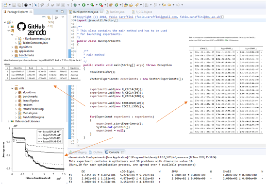
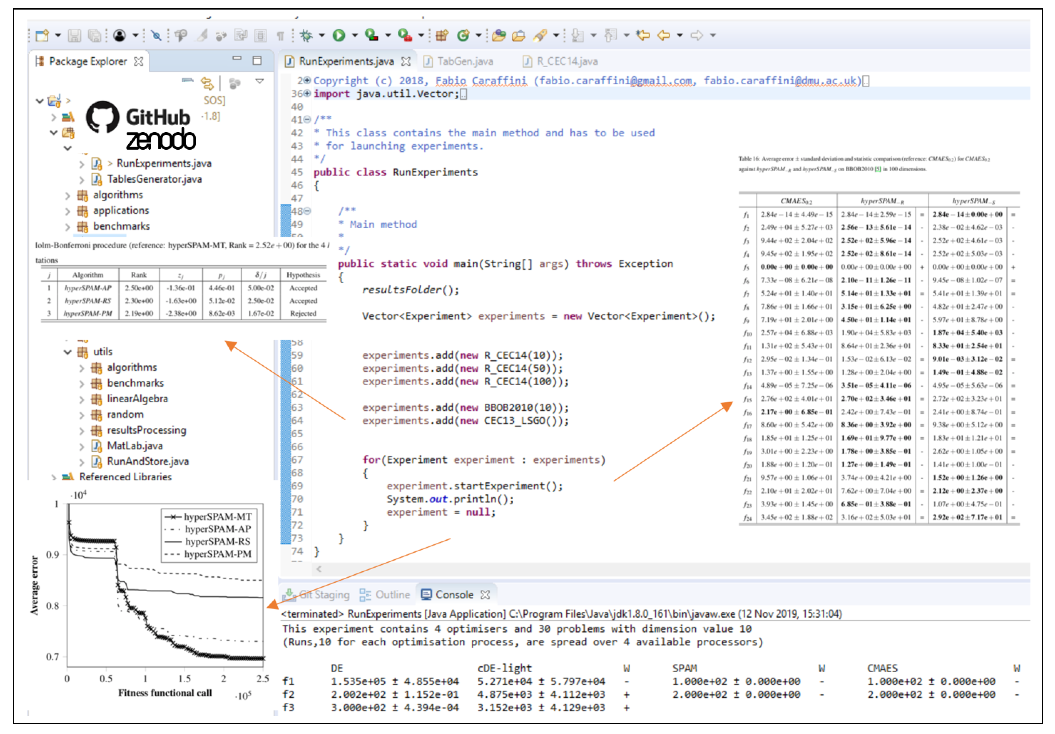
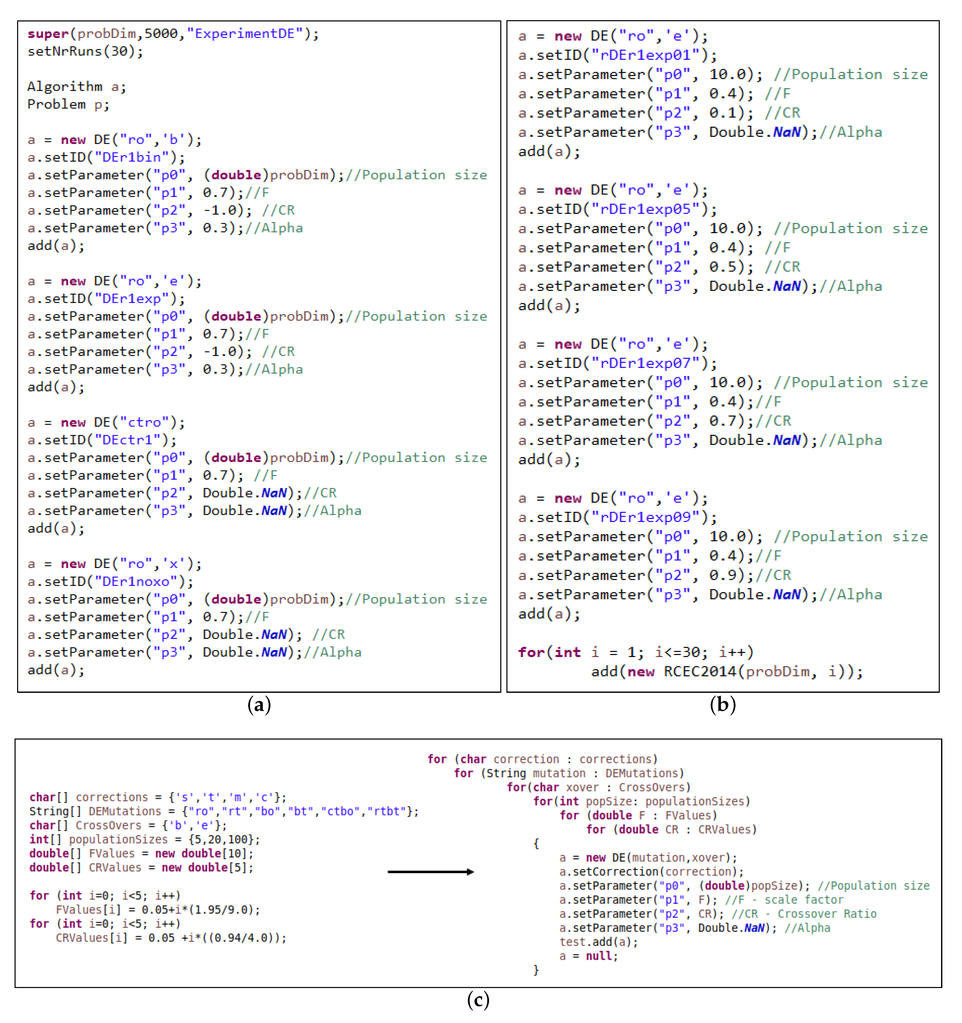
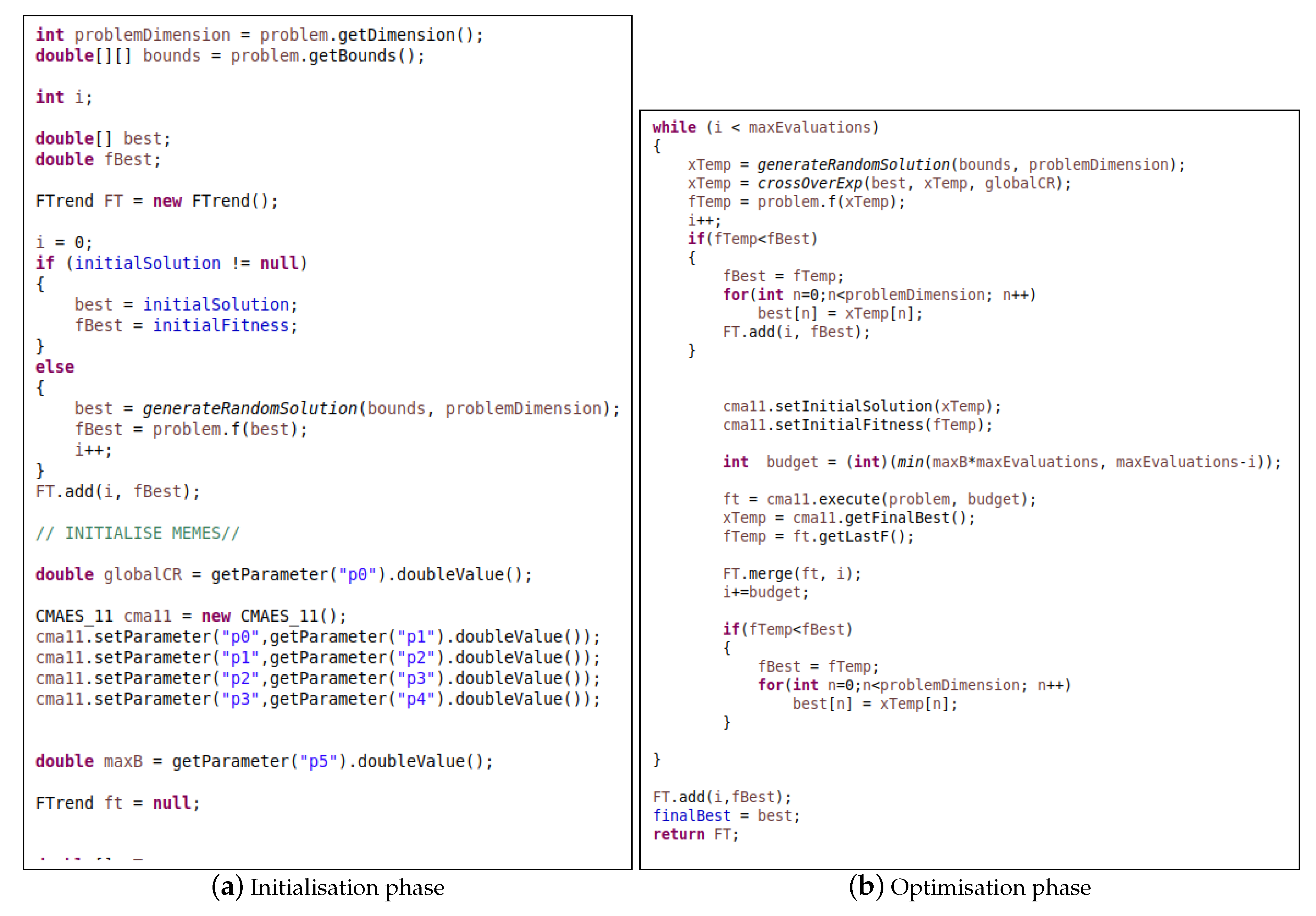
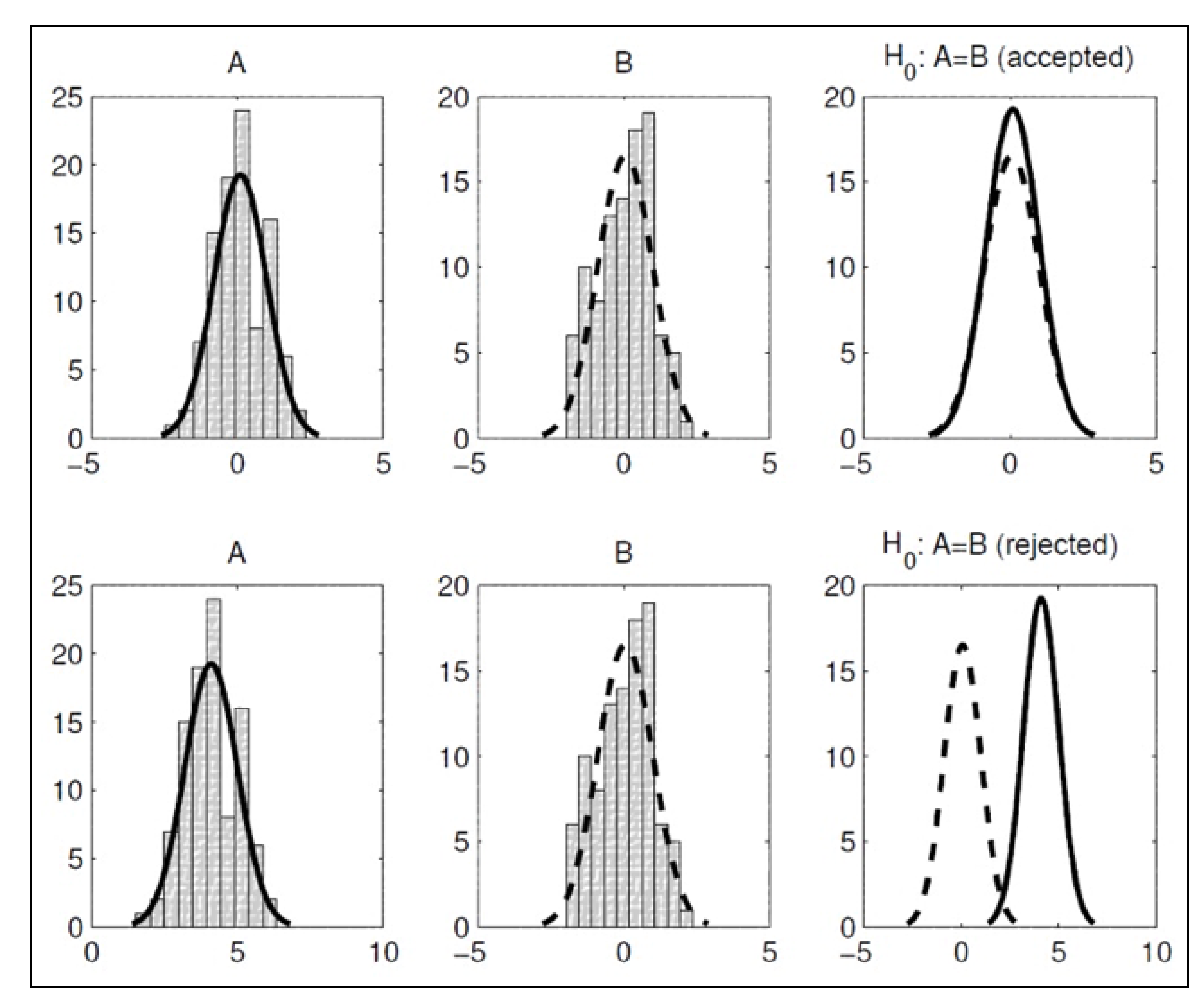
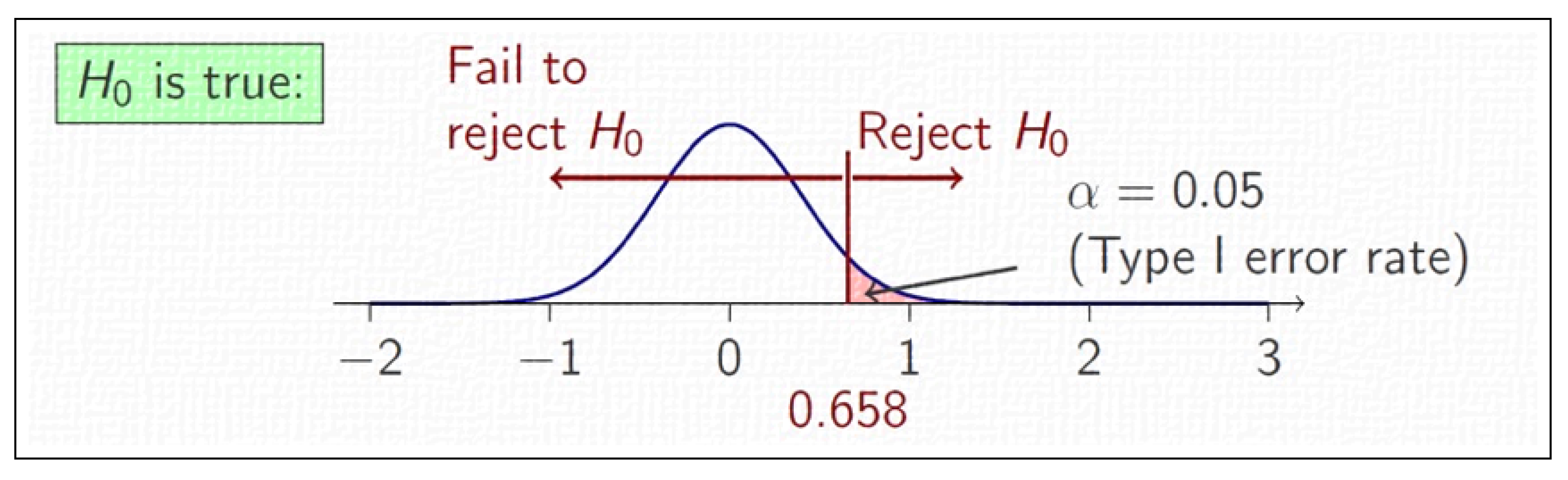
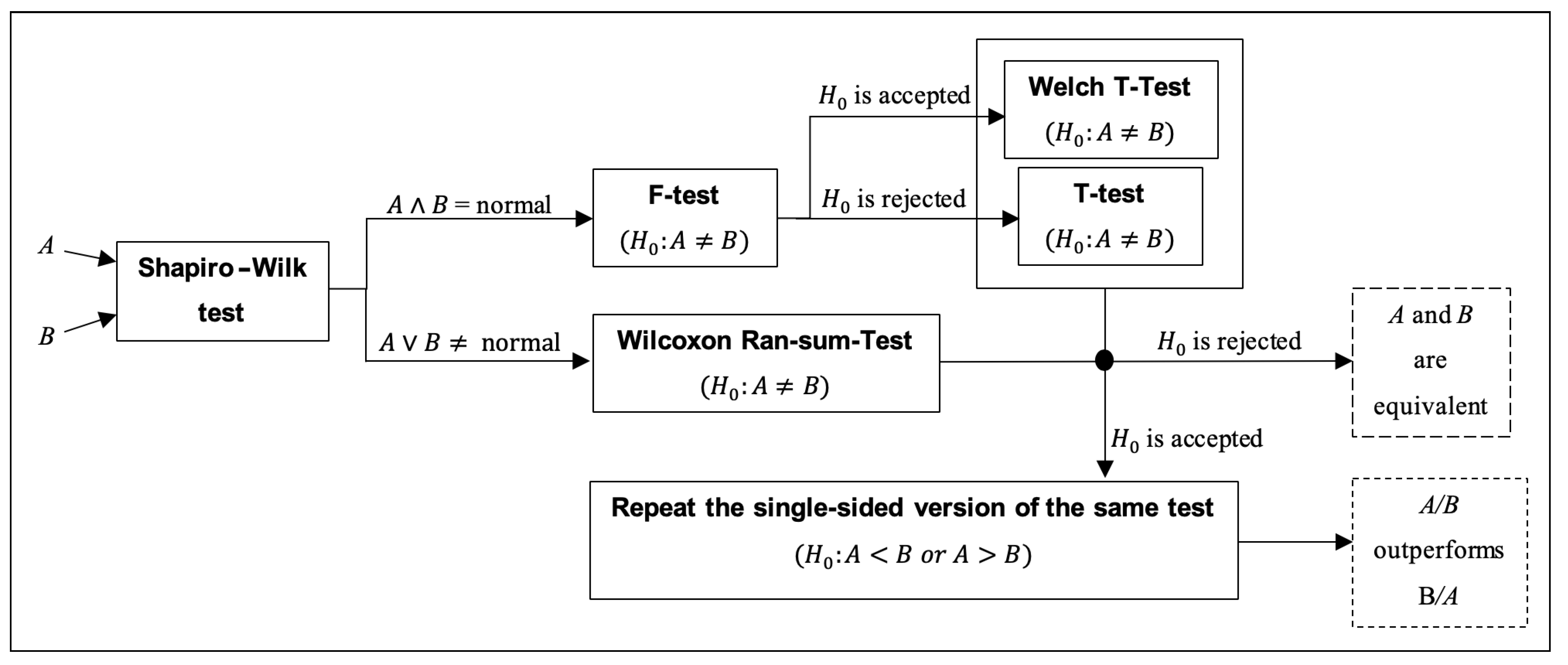
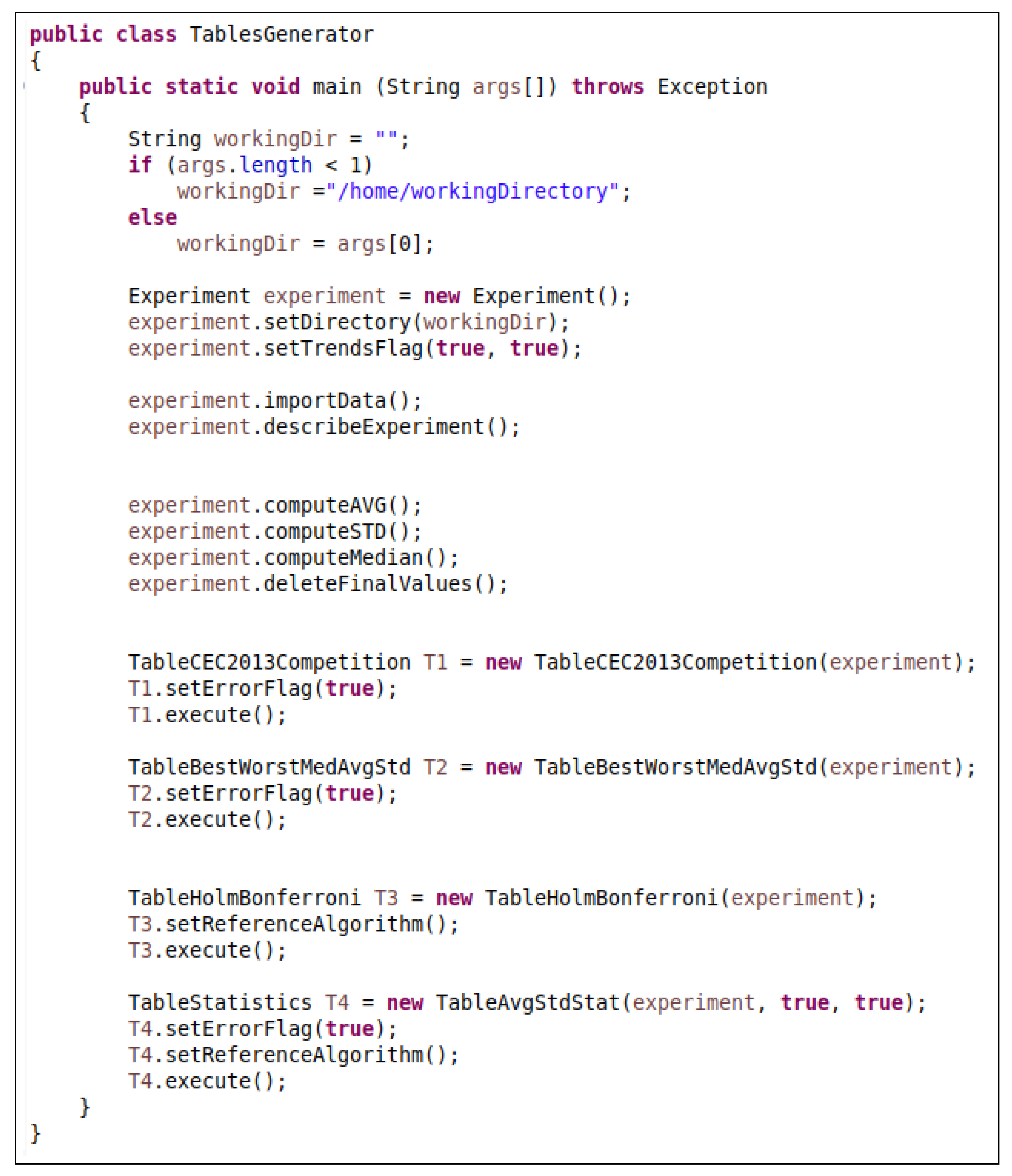
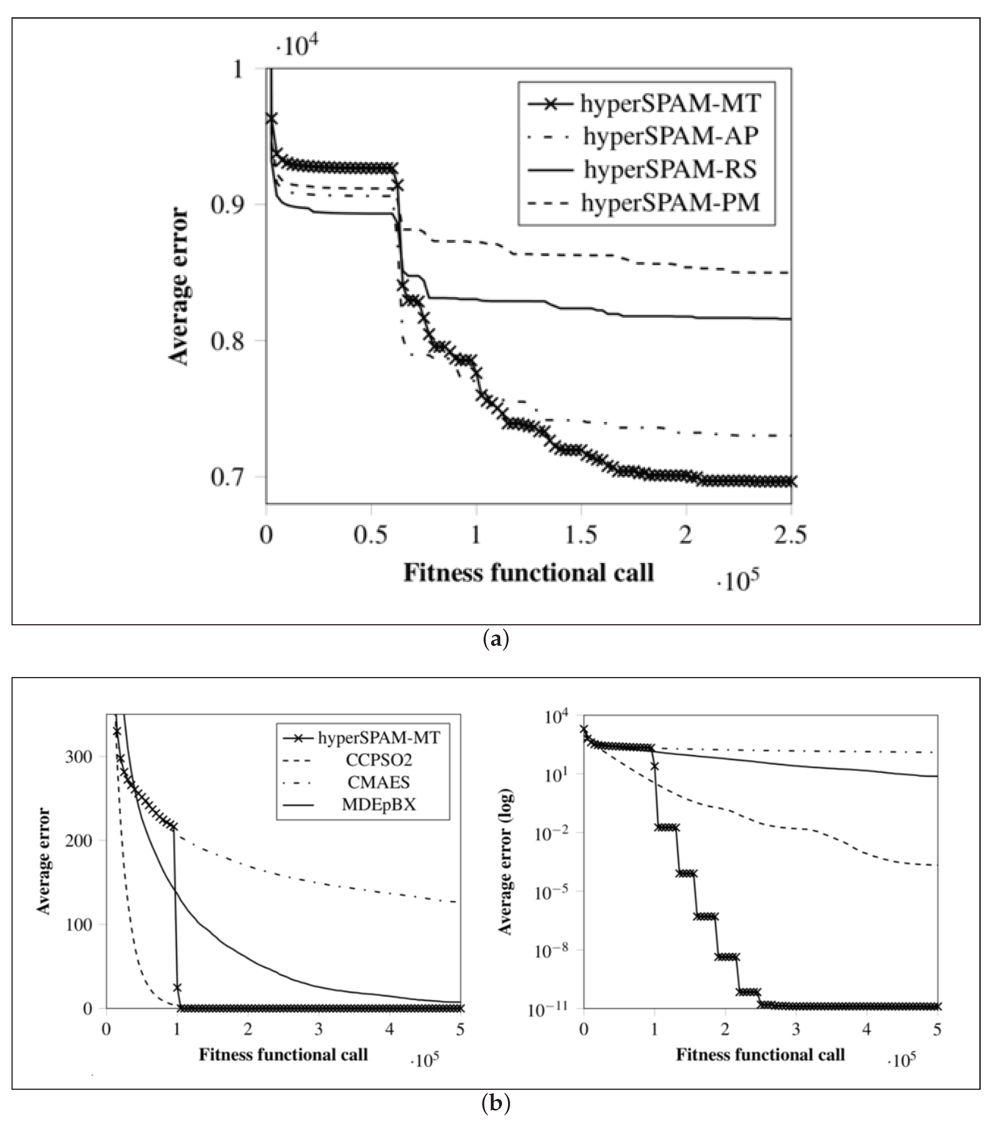
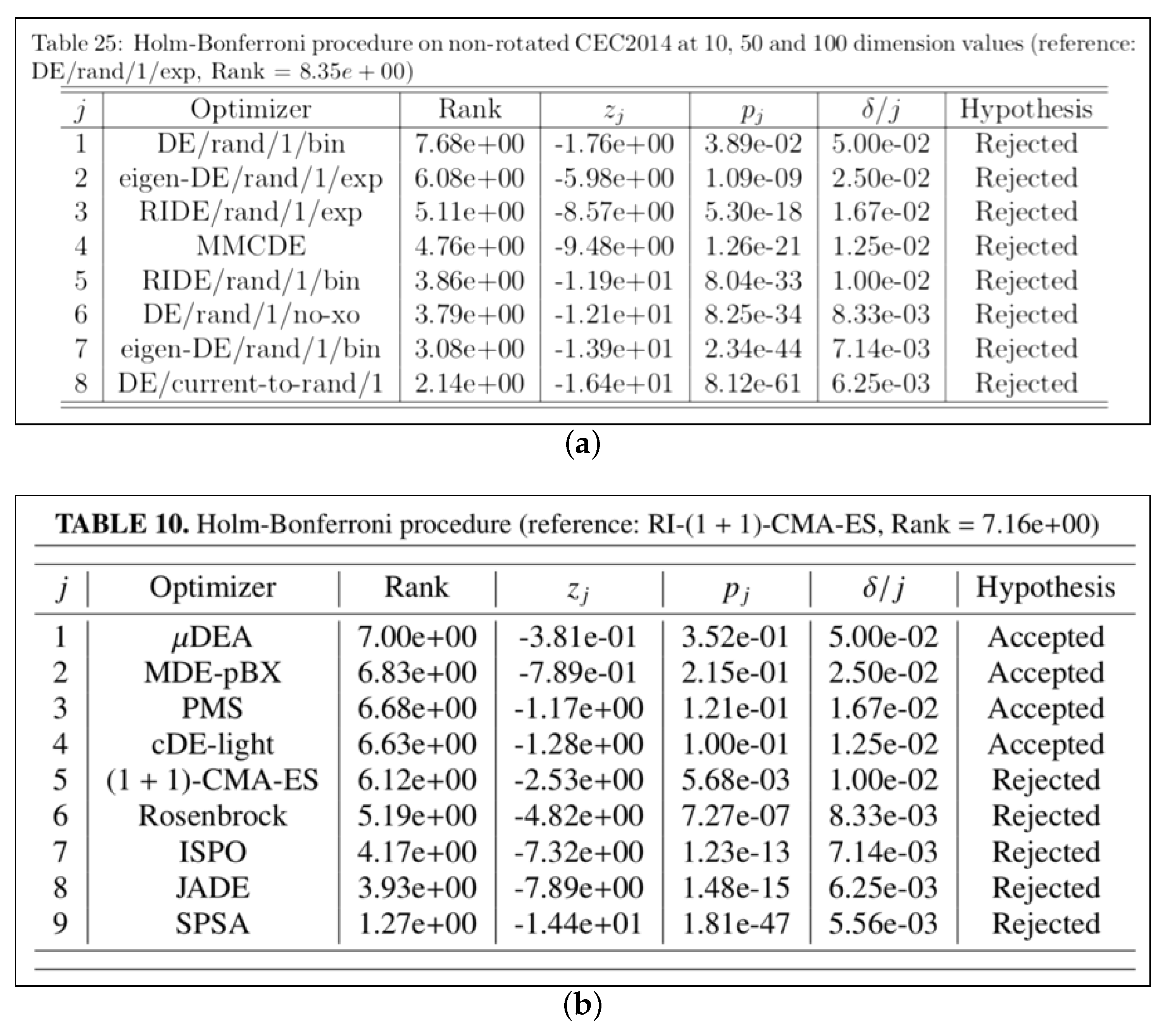
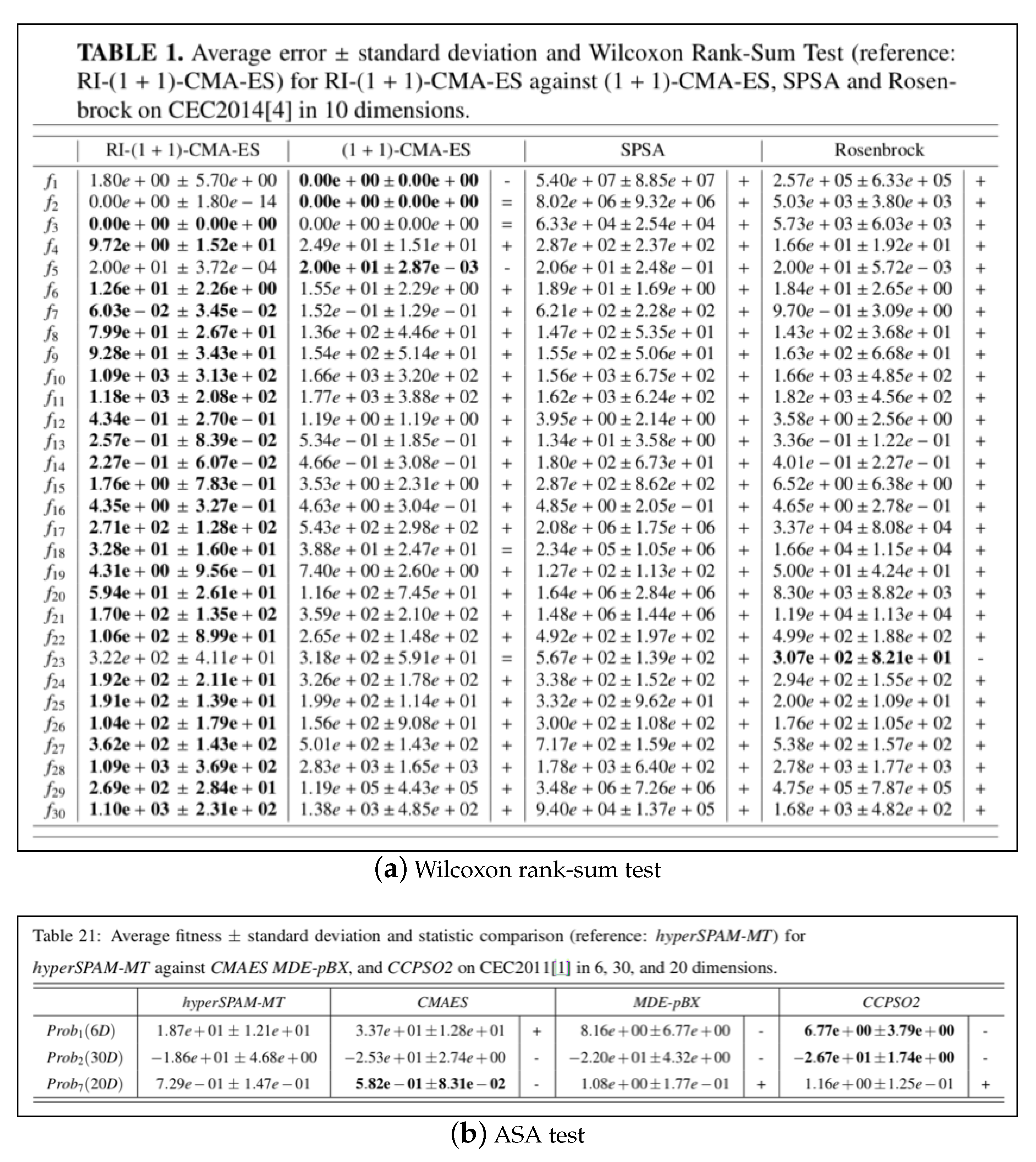
Table 1.
Relevant links to source code and software documentation.
| Description | Content | Link |
|---|---|---|
| SOS web page | software documentation | https://tinyurl.com/FabioCaraffini-SOS |
| GitHub repository | source code | https://github.com/facaraff/SOS |
| Zenodo repository [17] | SOS releases | https://doi.org/10.5281/ZENODO.3237023 |
Table 2.
R-CEC14 (R stands for rotation flag) benchmark suite. Each problem can be evaluated with and without the action of the rotation. Further details on these problems and the rotation procedure are available at [2].
Table 2.
R-CEC14 (R stands for rotation flag) benchmark suite. Each problem can be evaluated with and without the action of the rotation. Further details on these problems and the rotation procedure are available at [2].
| f Class | f Number | Function Name and Description | |
|---|---|---|---|
| Unimodal | 1 | High Conditioned Elliptic Function | 100 |
| 2 | Bent Cigar Function | 200 | |
| 3 | Discus function | 300 | |
| Multimodal | 4 | Shifted Ackley’s Function | 400 |
| 5 | Shifted Rosenbrock’s | 500 | |
| 6 | Shifted Griewank’s Function | 600 | |
| 7 | Shifted Weierstrass Function | 700 | |
| 8 | Shifted Rastrigin’s | 900 | |
| 9 | Shifted Schwefel’s | 1100 | |
| 10 | Shifted Katsuura | 1200 | |
| 11 | Shifted HappyCat | 1300 | |
| 12 | Shifted HGBat | 1400 | |
| 13 | Shifted Expanded Griewank’s plus Rosenbrock’s | 1500 | |
| 14 | Shifted and Expanded Scaffer’s F6 Function | 1600 | |
| Hybrid | 15 | Hybrid Function 1 | 1700 |
| 16 | Hybrid Function 2 | 1800 | |
| 17 | Hybrid Function 3 | 1900 | |
| 18 | Hybrid Function 4 | 2000 | |
| 19 | Hybrid Function 5 | 2100 | |
| 20 | Hybrid Function 6 | 2200 | |
| Hybrid | 21 | Composition Function 1 | 2300 |
| 22 | Composition Function 2 | 2400 | |
| 23 | Composition Function 3 | 2500 | |
| 24 | Composition Function 4 | 2600 | |
| 25 | Composition Function 5 | 2700 | |
| 26 | Composition Function 6 | 2800 | |
| 27 | Composition Function 7 | 2900 | |
| 28 | Composition Function 8 | 3000 |
Table 3.
Table of truth, also known as the confusion matrix.
| Is True | Is False | |
|---|---|---|
| Test rejects | Type I error | Correct inference |
| (False Positive) | (True Positive) | |
| Test fails to rejects | Correct inference | Type II error |
| (False Negative) | (True Negative) |
© 2020 by the authors. Licensee MDPI, Basel, Switzerland. This article is an open access article distributed under the terms and conditions of the Creative Commons Attribution (CC BY) license (http://creativecommons.org/licenses/by/4.0/).
Share and Cite
MDPI and ACS Style
Caraffini, F.; Iacca, G. The SOS Platform: Designing, Tuning and Statistically Benchmarking Optimisation Algorithms. Mathematics 2020, 8, 785. https://doi.org/10.3390/math8050785
AMA Style
Caraffini F, Iacca G. The SOS Platform: Designing, Tuning and Statistically Benchmarking Optimisation Algorithms. Mathematics. 2020; 8(5):785. https://doi.org/10.3390/math8050785
Chicago/Turabian StyleCaraffini, Fabio, and Giovanni Iacca. 2020. "The SOS Platform: Designing, Tuning and Statistically Benchmarking Optimisation Algorithms" Mathematics 8, no. 5: 785. https://doi.org/10.3390/math8050785
Note that from the first issue of 2016, this journal uses article numbers instead of page numbers. See further details here.