A Computational Investigation of Storm Impacts on Estuary Morphodynamics


Zienkiewicz Centre for Computational Engineering, College of Engineering, Swansea University, Swansea SA18EN, UK
*
Authors to whom correspondence should be addressed.
J. Mar. Sci. Eng. 2019, 7(12), 421; https://doi.org/10.3390/jmse7120421
Submission received: 4 October 2019
/
Revised: 8 November 2019
/
Accepted: 13 November 2019
/
Published: 20 November 2019
(This article belongs to the Section Coastal Engineering)
Abstract
:Global climate change drives sea level rise and changes to extreme weather events, which can affect morphodynamics of coastal and estuary systems around the world. In this paper, a 2D process-based numerical model is used to investigate the combined effects of future mean sea level and storm climate variabilities on morphological change of an estuary. Morphodynamically complex, meso-tidal Deben Estuary, located in the Suffolk at the east coast of the UK is selected as our case study site. This estuary has experienced very dynamic behaviors in history thus it might be sensitive to the future climate change. A statistical analysis of future storms around this area, derived from a global wave model, has shown a slight increase of storm wave heights and storm occurrences around the estuary in future as a result of global climate variations under medium emission scenario. By using a process-based model and by combining the forecast ‘end-of-century’ mean sea level with statistically derived storm conditions using projected storms over a time slice between 2075–2099, we determined hydrodynamic forcing for future morphodynamic modelling scenarios. It is found that the effect of increased sea level combined with future storms can significantly alter the current prevailing morphodynamic regime of the Deben Estuary thus driving it into a less stable system. It is also found that storm waves can be very significant to morphodynamic evolution of this tide-dominated estuary.
1. Introduction
Coastal morphodynamic systems, driven by coastal and oceanic forces such as sea levels, waves and surges, will be affected by future changes to global climate [1,2,3,4]. Estuaries, which are an integral part of coastal systems, may also undergo significant changes as a result. Apart from the potential losses of coastal wetlands and biological or ecological resources associated with estuaries [2], global climate change may affect sediment distributions and hence the morphology of these naturally complex systems.
Estuaries can be classified as either tide-dominated or wave-dominated morphodynamic systems. In tide-dominated estuaries, flood and ebb tidal processes govern sediment dynamics in and around the estuary thus shaping its morphodynamic characteristics. In wave-dominated estuaries, incoming waves, surges, and associated littoral transport processes dominate the morphodynamic regime. However, morphologies of most estuaries are largely shaped by the combined effects of waves, surges, and tides. Some estuaries may in fact switch between tide and wave dominance in their evolution histories. Thus, any potential changes to the incoming wave climate, specifically to storm wave conditions, as well as sea levels, can have significant implications on the future evolution of estuary morphology.
Although the impacts of slow changes to sea levels and incoming waves will be felt over a long period, occurrence of more intense and frequent extreme storm events as a result of global climate change may lead to change estuarine morphology over a very short time window. Extreme events may be able to alter static or dynamic long-term morphodynamic equilibria and force them into unstable morphodynamic regimes. For example, the onshore sediment transport into the Ribble Estuary (UK) is enhanced during storms which then have contributed to the rate of infilling of the estuary [5]. In the Humber Estuary in the UK, responses to storm surge have found to vary considerably, where some areas may accrete and others might erode as a result [6]. The North Sea storm surge of 1953 caused considerable flooding in the Deben Estuary, UK, which rapidly changed its shape, orientation, and location of the ebb delta [7]. Significant morphological changes had taken place as a result of combined extreme surge-wave-river flow conditions in Teign Estuary, UK [8]. Similarly, some notable morphodynamic changes observed in Seine Estuary and the Mont-Saint-Michel Bay in France have been attributed mostly to the enhanced storminess [9].
Storminess, however, which is termed as the combination of storm severity and frequency, has shown high spatial variability over the past decades, with a general pole-ward shift and increased intensity/decreased frequency of events around the UK [10]. As a result of future changes to the global climate, not only the sea levels have been predicted to increase but also the extreme storm conditions have been proven to be modified [11,12,13]. The intensity and frequency of the storms in most parts of the world have been reported to increase [2,14,15,16]. Future storms around some parts of the UK have been found to be changed, resulting in a change on either frequency or intensity of storms [13,17,18,19]. Seasonal extremes of significant wave heights in the North Atlantic have been analyzed based on a 40-year numerical wave hindcast by Wang and Swail [20], who found that the winter wave heights had been increased in the region northwest of Ireland but less significant changes in the North Sea. It has been found by Woth et al. [13] that storm surge extremes might increase for most of the North Sea coast. Wolf et al. [21] noted that there was a slight increase in the severity of the most extreme events while the frequency of extreme wind and wave events was slightly reduced generally in Liverpool Bay, UK, and in the same place, Brown et al. [22] concluded that the severity of most extreme wind and wave events would increase while frequency of storm occurrence would reduce in the future. These studies reveal that the UK coastline will be subjected to changes on intensity and frequency of extreme events to some degree in the future.
When considering the future climate conditions for estuaries, the sea level rise is one of the critical factors. Numerous studies have reported the impacts of sea level rise on estuarine morphodynamics. For example, Dissanayake et al. [23] numerically modelled Wadden Sea inlet using Delft3D computational suite [24] and reported that the flood delta volume of the inlet would increase while the ebb delta volume would decrease with the increased rate of future sea level rise (SLR). Karunarathna and Reeve [25] developed a behavior-oriented estuary morphodynamic model based on Boolean logic to predict estuary response to SLR. The application of the model to the Ribble Estuary revealed that the estuary would evolve into a new equilibrium as a result of SLR. Passeri et al. [26], using a numerical modelling study, concluded that hydrodynamics and hence morphodynamics of the Mississippi–Alabama barrier island were influenced by SLR. Recently, Yin et al. [27] investigated the effects of SLR on the meso-tidal, ebb-dominated Deben Estuary in the UK using a numerical model and concluded that the Deben Estuary inlet would become more dynamic as a result of SLR. Duong et al. [28,29] computationally modelled sea level rise and wave impacts on small tidal inlets located in a micro-tidal environment. They concluded that inlet stability and some key behavioral characteristics of inlet would change as a result of SLR.
Therefore, although numerous studies on the impacts of SLR or combined effect of SLR and change in average wave conditions on estuarine morphology have been reported, investigations into the combined effects of SLR and future storm conditions, which might be modified by climate change as discussed above, on estuaries are sparse. In this study, we use the Deben Estuary inlet, located in the east coast of the UK, as our study site to investigate the impacts of the combined effect of future sea levels and future extreme events on estuary morphodynamics, using a process-based numerical model. This model has been validated by Yin et al. [27], which was successfully applied previously the impacts of sea level rise on the same estuary.
2. The Study Site and Its Environment
The Deben Estuary, located in the east coast of the United Kingdom (UK) facing the North Sea, is selected as our case study site (Figure 1). The estuary is an integral part of the Suffolk coastline at the east coast of UK. It is one of the most dynamic spit-enclosed estuaries in the UK [30]. The estuary is tide-dominated however, the inlet of the estuary is shaped by the combined effects of tides and waves [31,32,33,34,35]. The mean spring tide range of the estuary varies from 3.2 to 3.6 m and it is therefore classified as meso-tidal estuary. The mean wave height at the mouth of the estuary is around 0.96 m with the predominant wave direction being north-east [34]. The inner estuary is morphodynamically stable while the estuary inlet is very morphodynamically active. The estuary has developed an ebb shoal which regularly changes its direction and length under strong tidal currents and the littoral regime [33]. The estuary inlet exhibits a cyclic morphodynamic evolution between three dominant morphodynamic states where the period of the cycles varies between 10 to 30 years [32,33]. It has been found that episodic high energy storm conditions alter these cycles. For example, the well-known 1953 storm in the North Sea appears to have driven a large quantity of sediment onshore to the downstream of the ebb delta [7]. A complex littoral sediment transport regime has been reported at the mouth of Deben Estuary with a long-term drift pattern driven by waves approaching the inlet predominantly from the north-east [32,33].
3. Methodology: Data Analysis and Numerical Modelling
3.1. Hyrodynamic Conditions Including Future Sea Level Rise and Storm Climate at Study Site
3.1.1. Sea Level
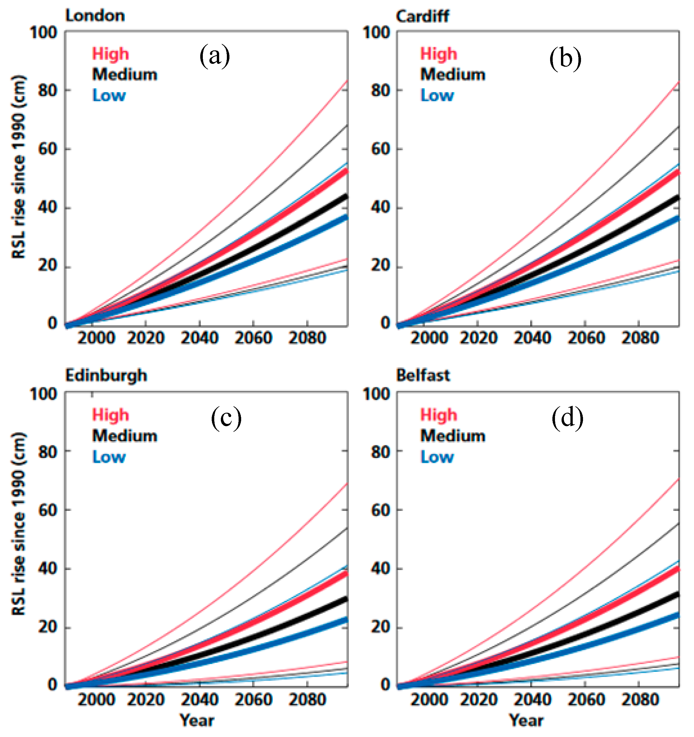
Sea level has risen globally during the last few hundred years due to global warming [14]. With the effect of long-term vertical land movement on regional sea level, the Relative Sea Level Rise (RSLR) at some locations can exceed global Mean Sea Level Rise (MSLR) by an order of magnitude [36]. Therefore, regional mean sea level changes may deviate from global trends. The UK Climate Projections (UKCP09) report has predicted mean sea level change around the UK under three emission scenarios: Low, medium, and high [14]. By combining the UK’s absolute time mean sea level change with isostatic and tectonic land movement estimates taken from [14], the RSLR at four UK sites (London, Cardiff, Edinburgh, and Belfast) have been reported in UKCP09, after taking into account the uncertainty of eustatic SLR (Figure 2). It has been reported that the northern part of UK has an uplift movement of the land while the southern part experiences lowering so that the RSLR rates in the south are slightly larger than that in the north [14].
In this study, the end-of-century mean sea level predicted for ‘London, UK’ under the medium emission scenario is used, considering the proximity of the study site to London. This matches with future wave projections carried out under A1B scenario in the Special Report on Emission Scenarios (SRES) in IPCC’s Fourth Assessment Report [37], which was used to determine future storm conditions in this study.
3.1.2. Waves
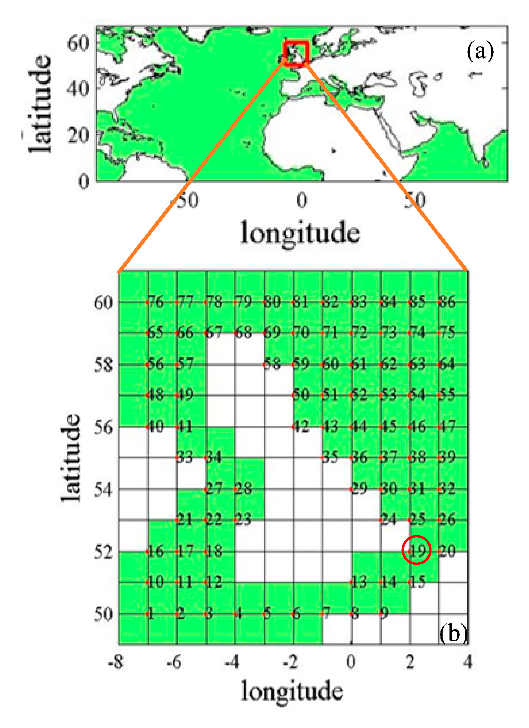
In this study, global wave projections carried out by Mizuta et al. [38] and Shimura et al. [39], using WAVEWATCH Ш model [40], taking sea surface wind from the Atmospheric General Circulation Model of the Meteorological Research Institute in Japan (MRI-AGCM3.2H), were used to determine the current and ‘end-of-century’ storm wave conditions. The global domain was set for the latitudinal range of 90°S–67°N over all longitudes with 1° × 1° spatial grids. The model has projected global climate for ‘present’ (1979–2009) and ‘future’ (2075–2099) time slices.
In ‘present (1979–2009)’ and ‘future (2075–2099)’ global ocean wave projections using 60 km resolution WAVEWATCH Ш model, four future statistically-analyzed sea surface temperatures (SSTs) have been defined as boundary conditions for MRI-AGCM3.2H [39,41]. However, our study only considers the first SSTs condition: the ensemble-mean SSTs projected by 18 models from phase 3 of the coupled model inter-comparison project (CMIP3) [15] under the A1B scenario from the Special Report on Emission Scenarios, which corresponds to the RSLR considered in this study. The global ocean wave model output nodes around the UK are shown in Figure 3.
The outputs of this global wave model provide three wave properties: Significant wave height (Hs), peak wave period (Tp), and mean wave direction (Dir) for two time slices: (i) Thirty years wave projections for the period 1979 to 2009 representing the current prevailing ocean wave climate (hereafter known as ‘present’ wave climate); (ii) 25 years wave projections between 2075 and 2099 representing the ‘end-of-century’ ocean wave climate (hereafter known as ‘future’ wave climate). Before using the projected wave data to determine storm conditions as wave forcing in the Deben Estuary morphodynamic model (Section 3.2), the model-derived waves under the ‘present’ climate time slice were validated against measured wave buoy data at “West Gabbard” WaveNet Site, (WGW), which is located at (51°58.96′N, 2°4.91′E) (Figure 1). Further details on this wave buoy, which is located in close proximity to Node 19 in Figure 3b, and its wave measurements can be found at CEFAS (https://www.cefas.co.uk/cefas-data-hub/wavenet/).
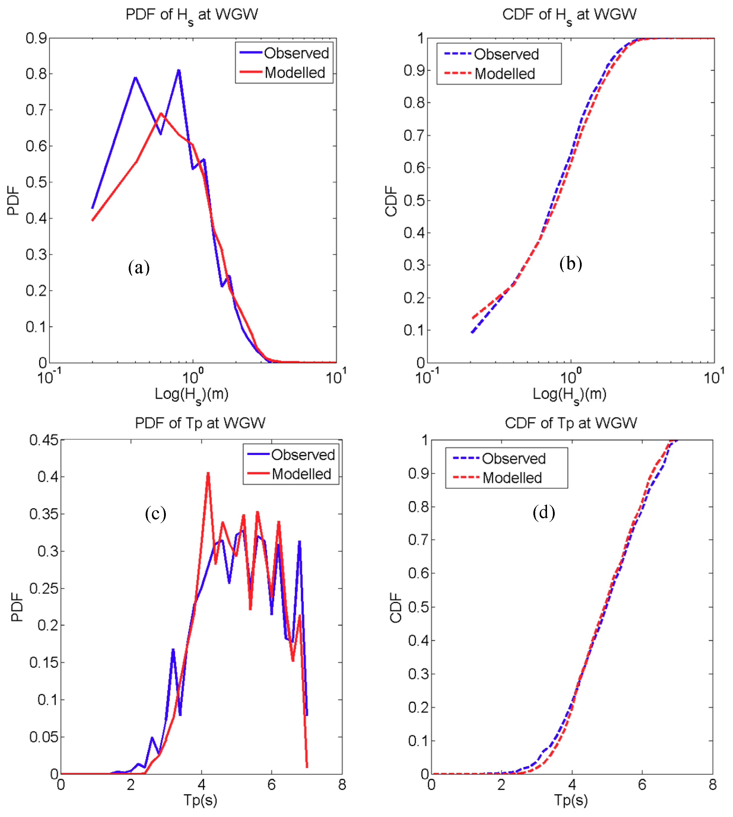
Measured wave data at WGW is only available from 2002 to 2009. Therefore, only the period between 2002 and 2009 are selected for validation of the global wave model. Empirical Probability Distribution Functions (PDF) and Cumulative Distribution Functions (CDF) of Hs and Tp of the modelled and measured wave heights are plotted in Figure 4. The results show that PDF and CDF of measured and modelled Hs and Tp at WGW are in good agreement.
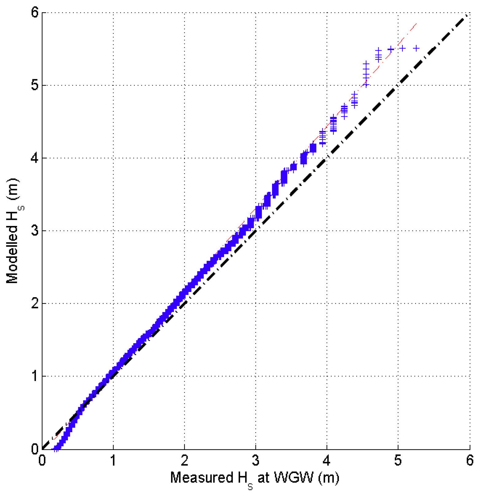
A quantile–quantile plot between the observed and modelled data sets with 1%–99% quantiles for Hs is shown in Figure 5. The quantile-quantile relationship between modelled and measured wave data is mostly linear around the diagonal line thus indicating good accuracy of wave height reproduction by the model. The model slightly underestimated smaller Hs values (average 20%) and overestimated large Hs values (average 10%).
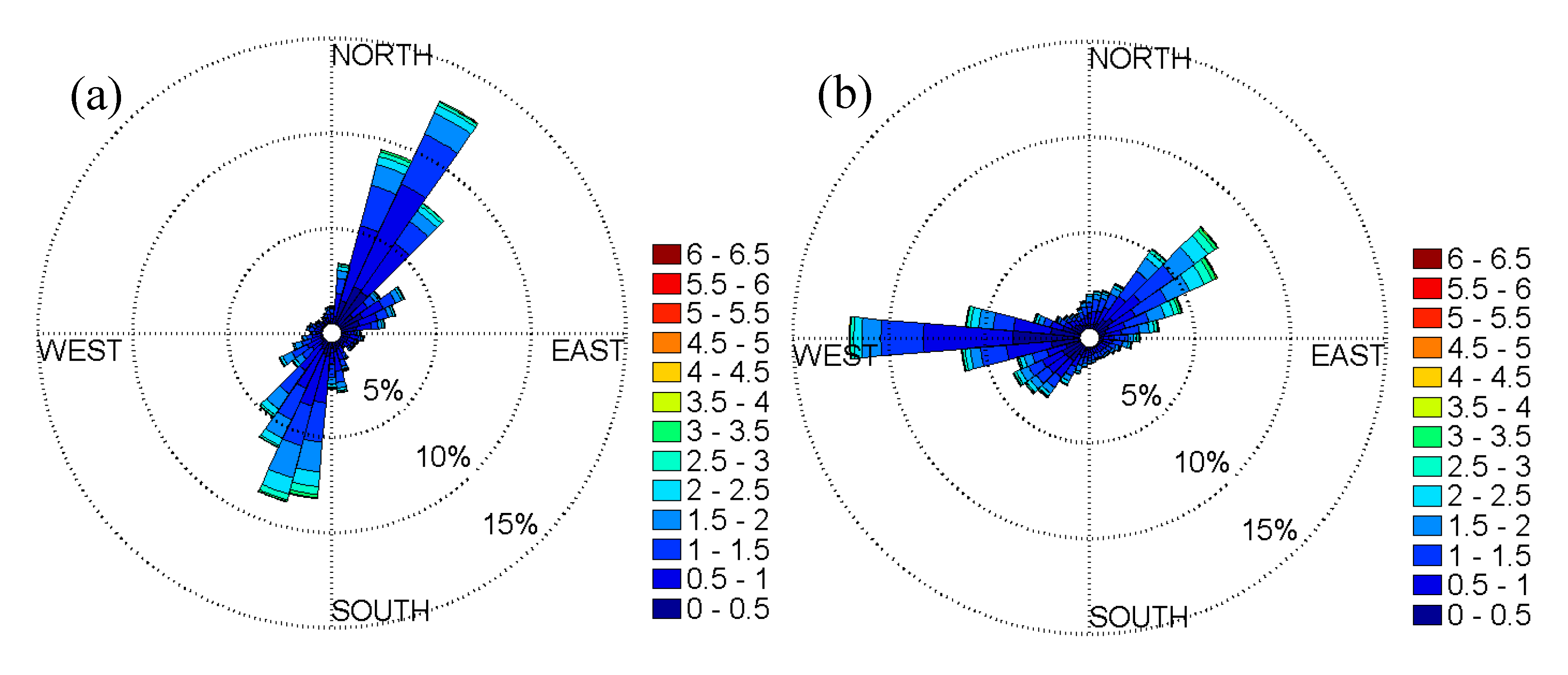
The predominant wave direction at WGW is north-east with more than 50% of the waves approaching from this direction (Figure 6a). Approximately 34.5% of incoming waves reached WGW from the south-westerly direction. The model was able to capture the north-easterly waves while most smaller waves have been projected with a westerly approach. It can be seen in Figure 6 that the global wave model correctly reproduced the approach directions of most waves with higher Hs values (north-east), which are the most important to the present study.
The mean absolute error, (MAE), between modelled and measured Hs and Tp are 0.68 m and 1.50 s, while the Root Mean Square Errors (RMSE) are 0.89 m and 1.87 s, respectively. For Hs values larger than 3.5 m, the average difference between modelled Hs and observed Hs is 0.11 m. The Hs values that are larger than 3.5 m in modelled and observed datasets are not available at the same timesteps and therefore it is not possible to determine RMSE values between them directly without interpolation. However, it should be noted that the percentages of Hs values larger than 3.5 m in both datasets are similar (2%–3%).
In summary, the global wave model was able to capture the prevailing wave climate offshore of the Suffolk coastline reasonably well while some disagreements were found in the wave directions. The deviations between modelled and measured Hs, Tp, and wave direction may be attributed to the level of resolution of the global wave model, wave–current interactions, local wave damping and other local effects, which are not captured in the global model and, also to the slightly different locations of model Node 19 and WGW site. However, we will only be using storm wave conditions in our simulations, where high energetic storm waves have been found to approach predominantly from the north-east. Therefore, some disagreements found between the measured and modelled wave directions will only have a minor impact on the results of our study.
3.1.3. Storms
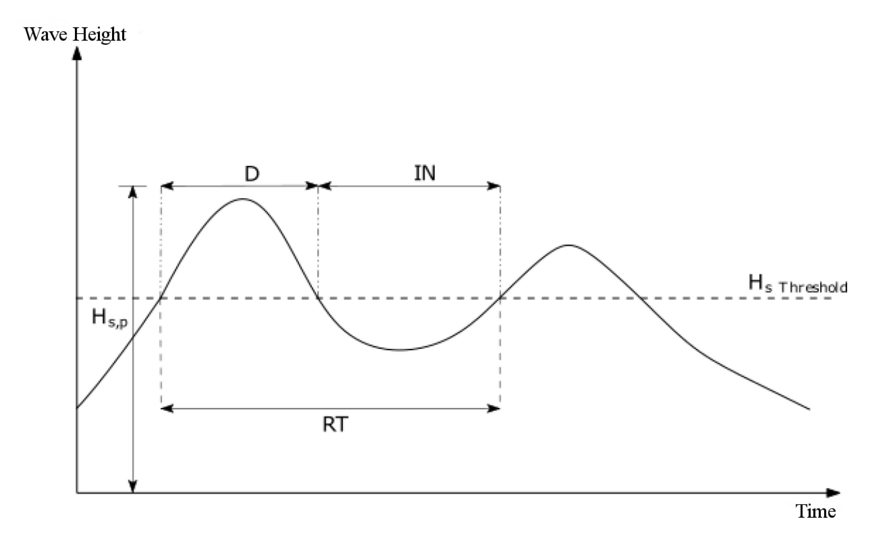
A storm event is defined as an event during which wave heights exceed a pre-defined threshold value for longer than a specified period. The pre-defined threshold wave height and the duration within which the wave heights are higher than the threshold can be site-specific and should be determined using historic wave data. If the time interval between two storms in a wave record is less than 24 h, then it is assumed to be one storm event with multiple peaks [42,43] (Figure 7).
Following the guidance provided by the UK Channel Coastal Observatory (CCO) and [43], we selected the threshold wave height Hs threshold of 2.5 m as our first guess. This gave us 724 storms from the projected wave height time series between 1979 and 2009 (‘present’ scenario) and 578 storms during 2075 to 2099 (‘future’ scenario). These storm data (peak storm wave heights) were then fitted into a Generalized Pareto Distribution (GPD) (Equations (1) and (2)), which can be used to identify an accurate site-specific storm wave height threshold as follows [44]:
in which u is the distribution threshold, Fu(y) represents the probability that the value of x exceeds u by amount of y, where y = x–u.
The cumulative distribution function (CDF) of GPD is expressed as:
where k is the shape parameter, β is the location parameter, α is the scale parameter.
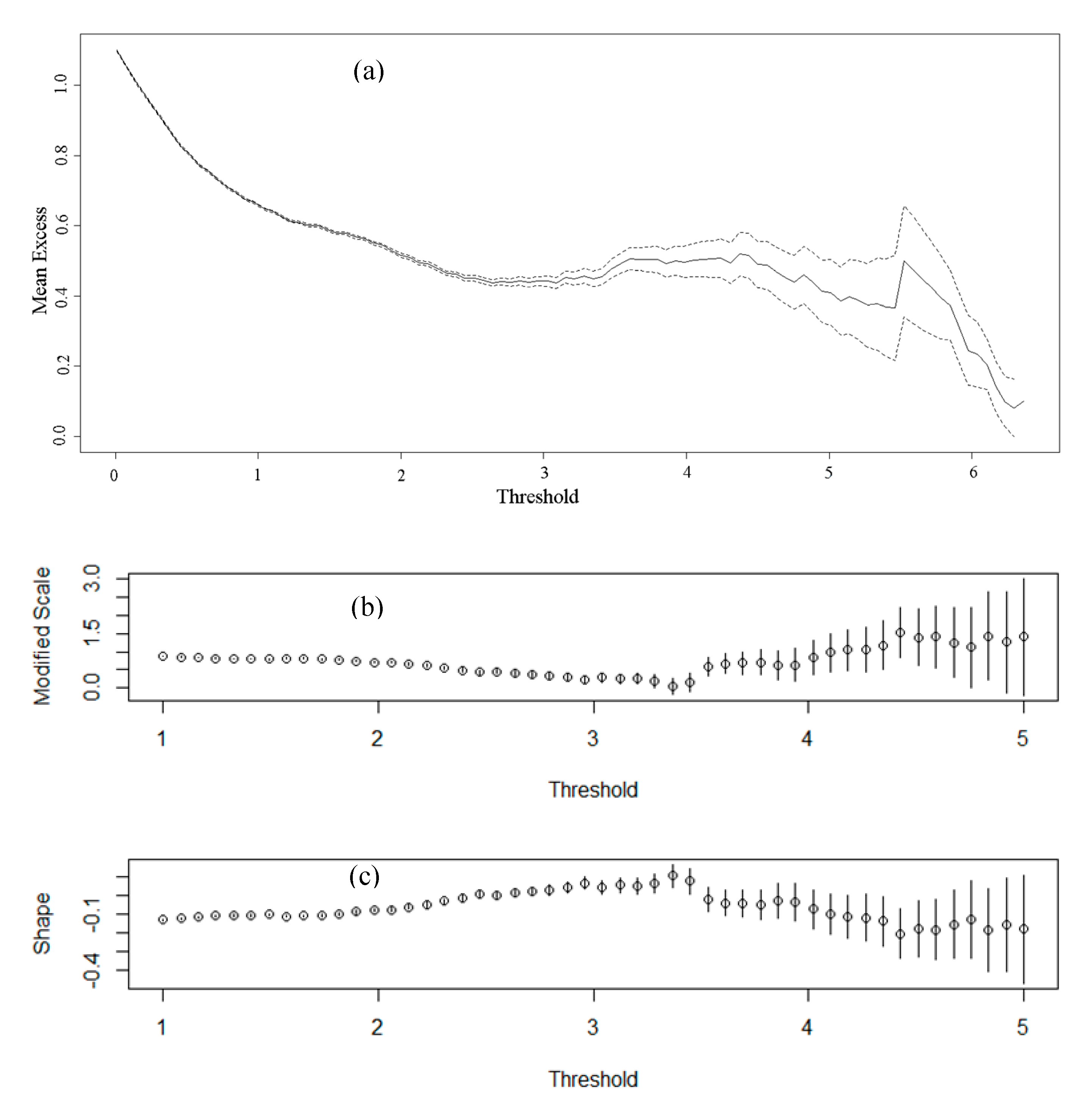
If the GPD is valid for excesses of the threshold u0, it should equally be valid for all thresholds u > u0. To determine the storm wave height threshold from GPD distribution, the Conditional Mean Exceedance (CME) graphs known as Mean Residual Life (MRL) plots, which show the relation between the threshold values and the mean excess over thresholds, is used [44,45]. The MRL plot based on the ‘present’ Hsmax values is shown in Figure 8. Since there is no significant difference between ‘present’ and ‘future’ Hsmax MRL plots, it is decided to use the same storm wave height threshold for both ‘present’ and ‘future’ storm conditions.
According to Coles [44], it is reasonable to determine the threshold above which the two variables (threshold and mean excess) are roughly linear with each other. It is found in Figure 8 that the two variables are nearly linear after Hsmax = 3.5 m. Therefore, 3.5 m is used as the storm threshold wave height to isolate storm from the ‘present’ and ‘future’ wave height time series. As stated by Coles [44], it may be difficult to use MRL plot as a method of threshold selection at some instances. At those situations, the threshold choice revisited process is required to look for stability of the parameter estimates. The middle and bottom figures in Figure 8 show that the variations for higher thresholds are large, but these perturbations are far smaller than sampling errors (vertical lines in these figures). Therefore, the selected threshold of 3.5 m is reasonable.
The selected threshold isolated 138 storms during 1979 to 2009 and 130 storms during 2075 to 2099. Table 1 shows the regressive peak storm wave heights (Hsmax) corresponding to several return periods, regressed from threshold GPD distribution for ‘present’ and ‘future’ conditions.
It can be seen that the ‘future’ storm wave heights are only slightly higher (around 3%) than ‘present’ storm wave heights at this site. However, this difference can make changes to the maximum storm wave heights corresponding to different return periods. For example, the 1 in 30-year return period of a storm with Hsmax = 6.11 m in the ‘present’ scenario might become 1 in 20-year return period storm in ‘future’ scenario (Hsmax = 6.12 m), which can be significant in the context of storm occurrence. In this paper, the 1 in 100-year storm for both ‘present’ and ‘future’ climate conditions were selected to investigate the impacts of global climate variabilities on morphodynamics of the Deben Estuary as 1 in 100-year event is considered for most coastal defences designs, flood management, and coast conservation purposes.
3.2. Numerical Modelling
3.2.1. Model Set Up
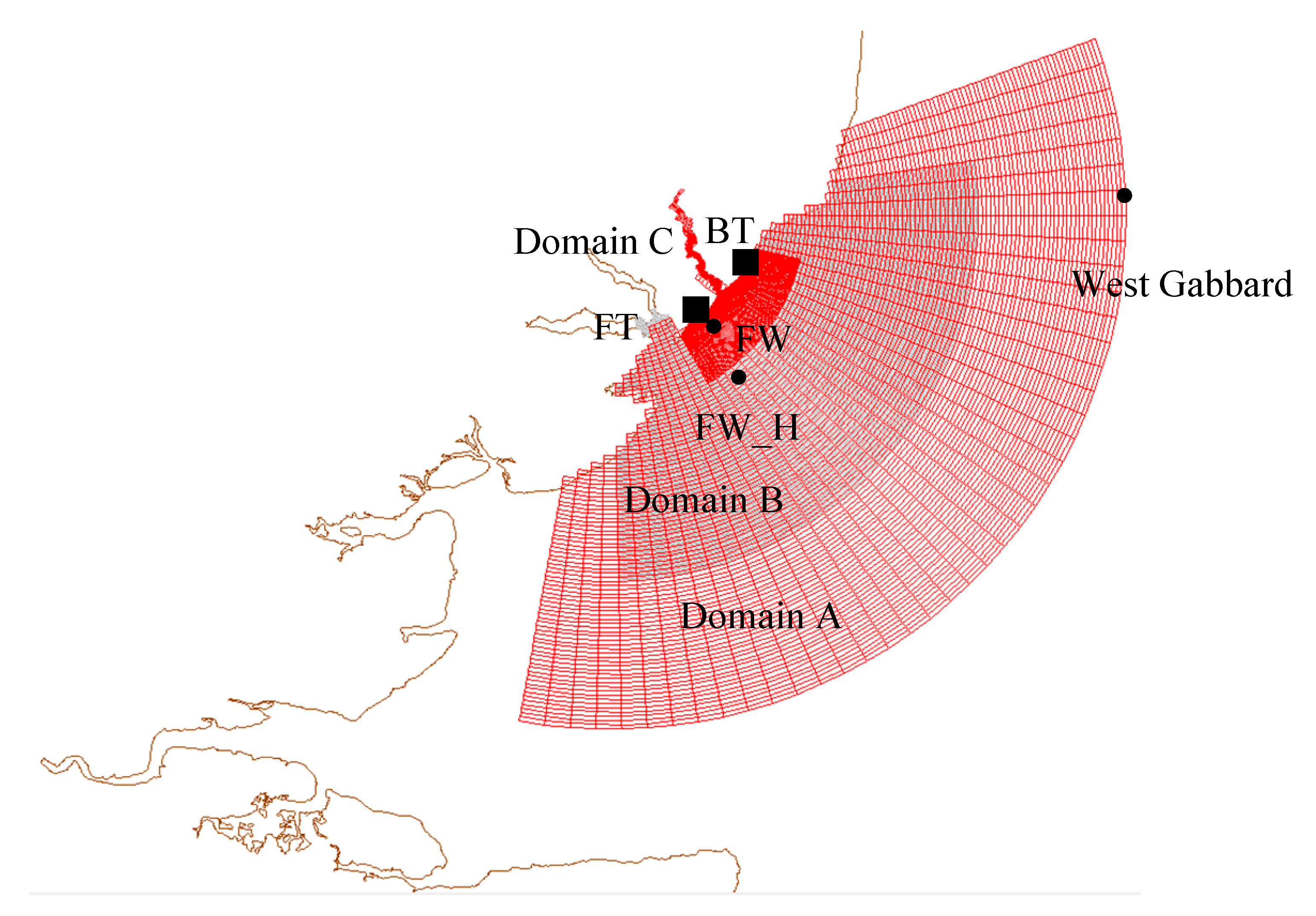
In this study, the process-based numerical modelling software Delft3D [24,46] is used to establish a numerical model of the Deben estuary and the surroundings (Figure 9). The model includes coupled flow and wave modules and, sediment transport and bed updating modules for morphodynamic prediction. Nested computational domains were used to achieve computational efficiency and required accuracy [27]. Within the smallest domain (Domain C in Figure 9), a domain decomposition process is implemented to achieve a higher resolution to resolve the morphodynamic changes within the estuary. Grid resolution of domains A, B, and C varied from 700 to 100 m. The shape of the offshore boundary of Domain A was designed to capture waves approaching from all directions. The offshore boundary passes through the WGW wave buoy position and it is assumed to correspond to Node 19 of the global model (Figure 3b). The tidal boundary conditions for the largest domain (Domain A) were determined from TPXO7.2 Global Inverse Tide model (from Oregon State University: http://volkov.oce.orst.edu/tides/TPXO7.2.html). Larger computational domains provided boundary conditions for the smaller domains. Only the smallest domain included morphological changes in which the sediment characteristics varied spatially, based on sediment measurements available for the Deben basin [32,33]. Considering the nature of sediment presented in the estuary, the Bijker [47] sediment transport formula is used for sediment transport calculations after a careful calibration [27]. The wave and tidal models were calibrated and validated by using the data from tide gauges, wave buoy measurements, and wave hindcasts (separated WAVEWATC III model) at several locations within the model domains. The square and circle dots in Figure 9 indicate that tidal and wave measurement locations used to validate the model [27]. As it is known that the inner estuary remains largely unchanged compared to the inlet region [32], our study is focused only on the Deben Estuary inlet region.
3.2.2. Model Validation
The model validation process was carried out using hindcast wave data and measured water levels in September of 2002. The Mean Absolute Error (MAE) and Root Mean Square Error (RMSE) values between measured and modelled water elevations at station FT are 0.24 and 0.31 m while that at station BT are 0.06 and 0.08 m, respectively. This represents a 6% and 2% difference between measured and modelled tidal amplitudes at FT and BT, respectively, which indicates the ability of the model in accurately reproducing tidal elevations [27]. The MAE and RMSE values between measured and modelled significant wave heights at FW site are 0.14 and 0.19 m, respectively and at hindcast site FW_H are 0.27 and 0.37 m, respectively. The slightly higher errors at FW_H may be partially attributed to the resolution of the WAVEWATCH Ш wave hindcast model, which may not be accurate enough to derive waves in shallow water [27]. For morphodynamic model validation, modelled bathymetry changes of the estuary between 2002 and 2003 was compared with the measured bathymetry changes between 2002 and 2003 bathymetry maps. The model correctly reproduced morphodynamic change of most areas of the inlet during this year except in the down-drift areas of the ebb delta. The differences can be attributed to lack of sediment supply (not included in the model but exist in real) to the domain from updrift areas of the inlet [27]. The detailed model set up and extensive model validations can be found in [27,48]. It should be noted that the pre- and post-storm estuary bathymetries are not available for morphodynamic model validations on storm impacts. Successful validation of the model gives confidence in using the model for investigating morphodynamic change of the Deben Estuary during storm events.
3.2.3. Storm Wave Conditions
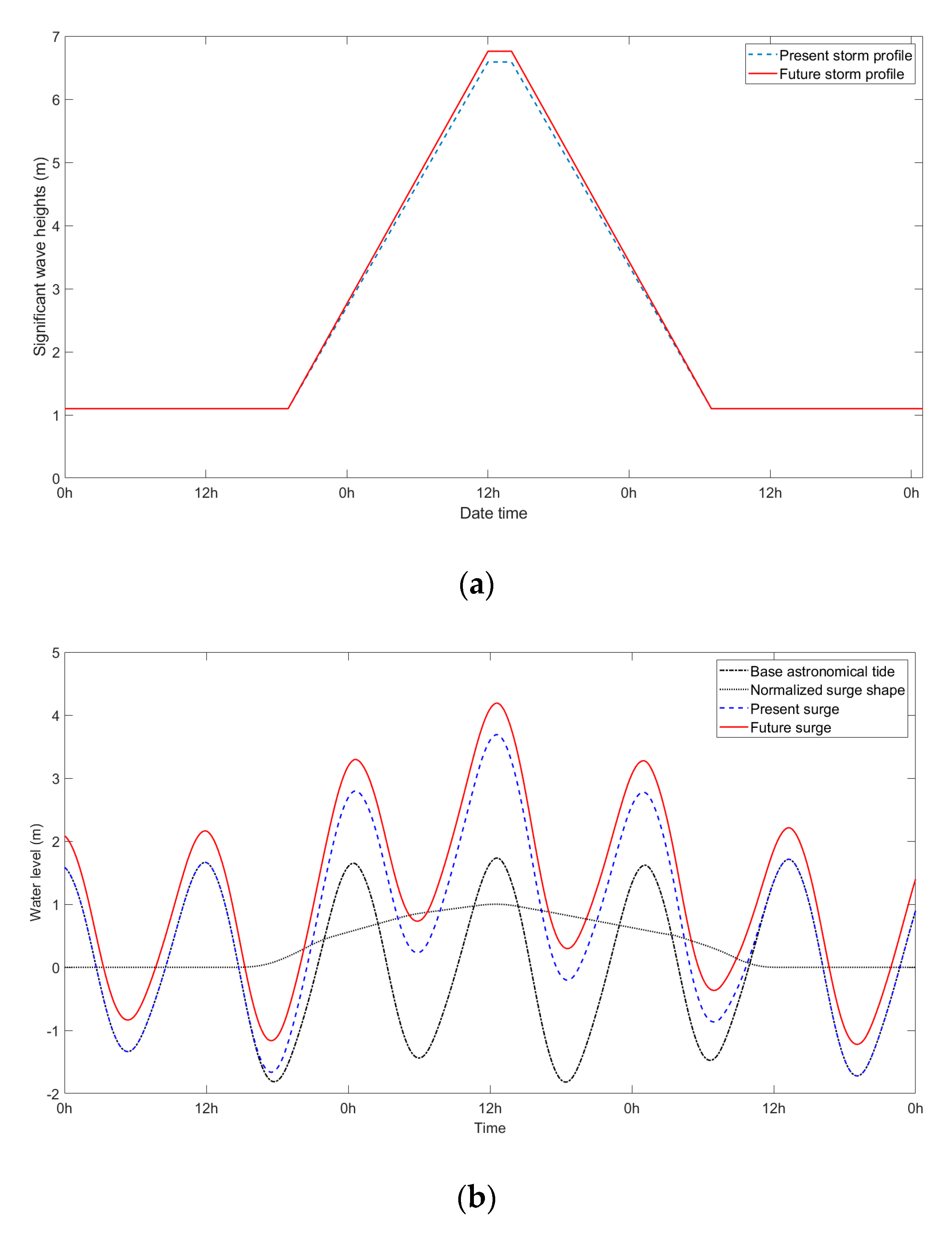
As mentioned above, we selected 1 in 100-year return period ‘present’ and ‘future’ storm condition to investigate the impacts of extreme storms on estuary morphodynamics. The peak wave period of the 1 in 100-year storm was determined using the relationship Tpmax = 5.3 × Hsmax 1/2 [49]. The duration of the storm was determined from a statistical analysis similar to that used to determine Hsmax, using storm durations isolated from the projected wave height data. The predominant wave direction of high energy wave approach (45°N) is used as the storm approach direction. An idealized trapezoidal storm profile was created based on Hsmax and storm duration (Figure 10a). Local spatially constant and temporally varied storm wind field of the study site, determined from the UK Met Office, is used by conducting an extreme value analysis of wind conditions similar to the extreme analysis carried out for wave data above.
In this model, the depth-induced wave breaking is considered by using the bore model of Battjes and Janssen [50] in which the total rate of dissipation depends critically on the breaking parameter, which depends on the water depth. The online-coupled interaction between tides and waves is also included in the modelling.
3.2.4. Storm Surge Conditions
The peak water level and the time-varying water level profiles are determined from the combination of the astronomic tides and extreme water level values associated with predicted surge profiles, following the method from McMillan et al. [51]. The overall extreme sea levels with a range of probabilities have been determined by McMillan et al. [51] using the skew surge joint probability method, (SSJPM), for 40 of the UK national network of (Class A) tide gauge sites from around the coastlines of England, Scotland, and Wales, together with equivalent data from five other primary sites, supplied by the National Tide and Sea Level Facility of the UK, (NTSLF). They also provided standardized surge profile at each tide gauge site [51].
Extreme water levels for a range of return periods, determined following McMillan et al. [51], are listed in Table 2. The standard storm surge profile used in this study is shown in Figure 10b. The estimated extreme water level did not include the local increase in sea level due to wave set up. The total water level includes the astronomical tide and the storm surge only.
The 1 in 100-year storm condition was assumed to coincide with the highest astronomical tide to generate the ‘worst’ case 1 in 100-year storm scenario. The total water level profile was derived by adding the time-varying surge profile to the base astronomical tide curve. The shape of the 1 in 100-year surge profile was created using the method described by McMillan et al. [51]. First, a scaling factor was determined using the difference between 1 in 100-year return period peak sea level (predicted by McMillan et al. [51]) and highest astronomical tide (from TPXO7.2). Then, the scaling factor was applied to the normalized surge shape shown in Figure 10b to create the actual surge profile. Finally, the surge profile was added to the astronomic tide level to determine total water level (Figure 10b).
In a changing climate it is possible that changing storminess will alter surge characteristics. However, it is difficult to forecast such changes with any assurance [10,36]. Therefore, we assumed the present surge profile remains unchanged in the future. SLR due to global warming is taken into account, which alters the total water level under ‘future’ climate scenario. The constructed storm wave heights and water level profiles are shown in Figure 10.
Model simulations were carried out for a three-day period during spring tide where the maximum spring high tide occurs 36 h after starting the simulation. The designed storm wave profile and water level conditions are shown in Figure 10 in which the storm profile increases from average wave height which is about 1.1 m to the extreme 1 in 100-year return period Hsmax then decreases to the mean wave height. The peak storm wave is corresponding to the peak water level. The first sixteen hours of the simulation are taken as a warm-up period of the simulation.
All scenarios are categorized into two groups: (i) ‘Present’ climate scenario where 1 in 100-year return period ‘present’ storm and surges are applied, (ii) ‘Future’ climate scenario where 1 in 100-year return period ‘future’ storm and surge together with the end-of-century SLR determined from medium emission climate change scenario are applied. In all simulations, it is assumed that the storm and the surge peak at highest spring tide thus generating the ‘worst’ case scenario.
3.2.5. Estuary Bathymetries
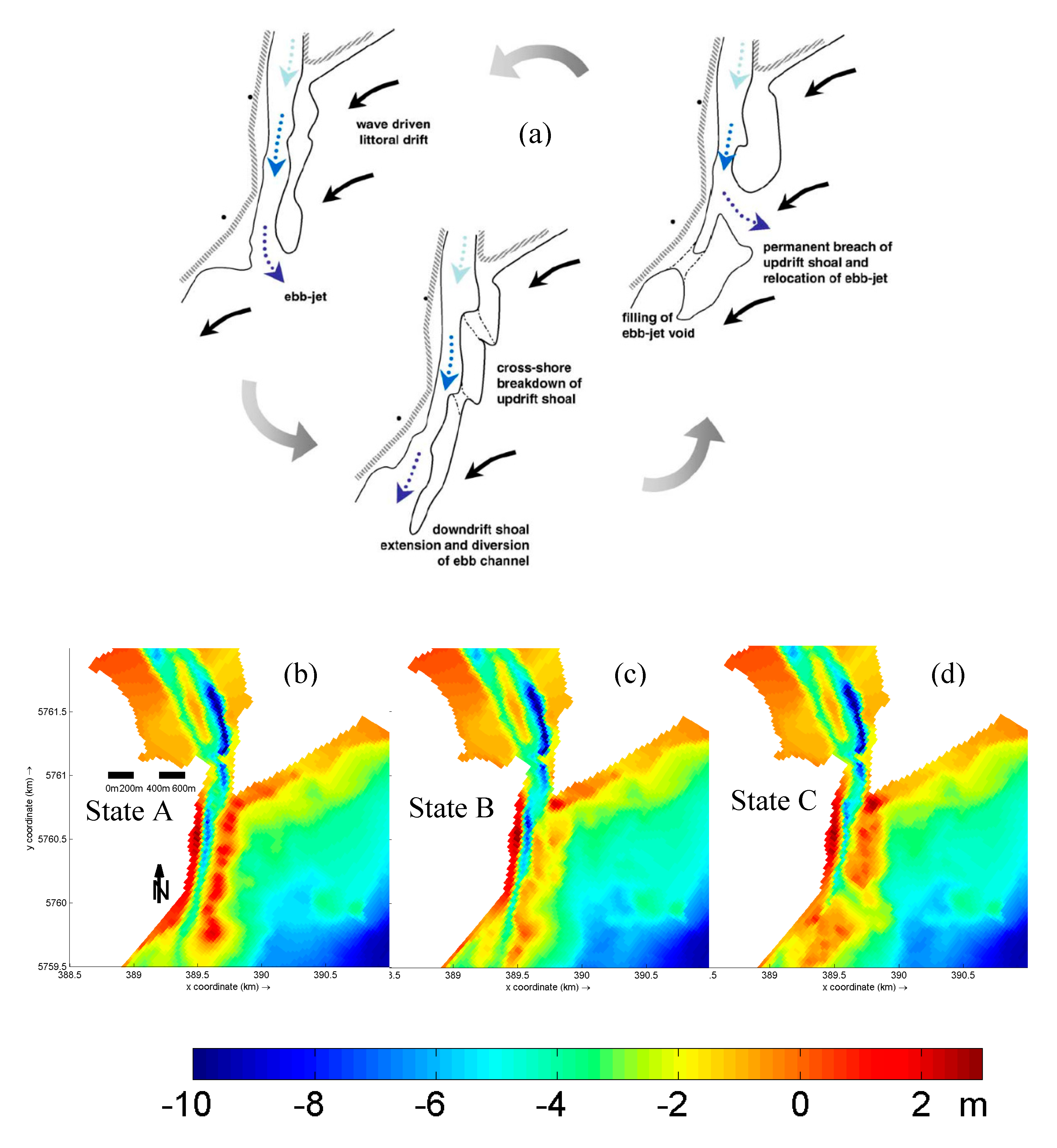
Historic bathymetry measurements of the Deben Estuary reveal that the inlet of the estuary exhibits three distinct morphological states between which it evolves cyclically [32], as mentioned in Section 2. Those three bathymetry states are shown in Figure 11. State A is the morphology associated with the progressive extension of the updrift ebb-tidal shoal causing down-drift migration of the ebb jet and some recession of the down drift shoreline. In State B, cross-shore breakdown of the updrift shoal, downdrift shoal extension, and diversion of the ebb channel are seen. State C has relocated the ebb jet region to a northerly position because of a permanent breach of the updrift shoal. It is possible that the estuary may be in any one of the above three states when a storm arrives. Morphodynamic modelling of the responses of the estuary to present and future storms were modelled taking all three morphodynamic states as initial bathymetries, which allows us to identify the most unstable post-storm inlet bathymetry. All modelled scenarios in this study are summarized in Table 3.
4. Results and Discussions
4.1. Estuary State A
4.1.1. Waves and Hydrodynamic Changes
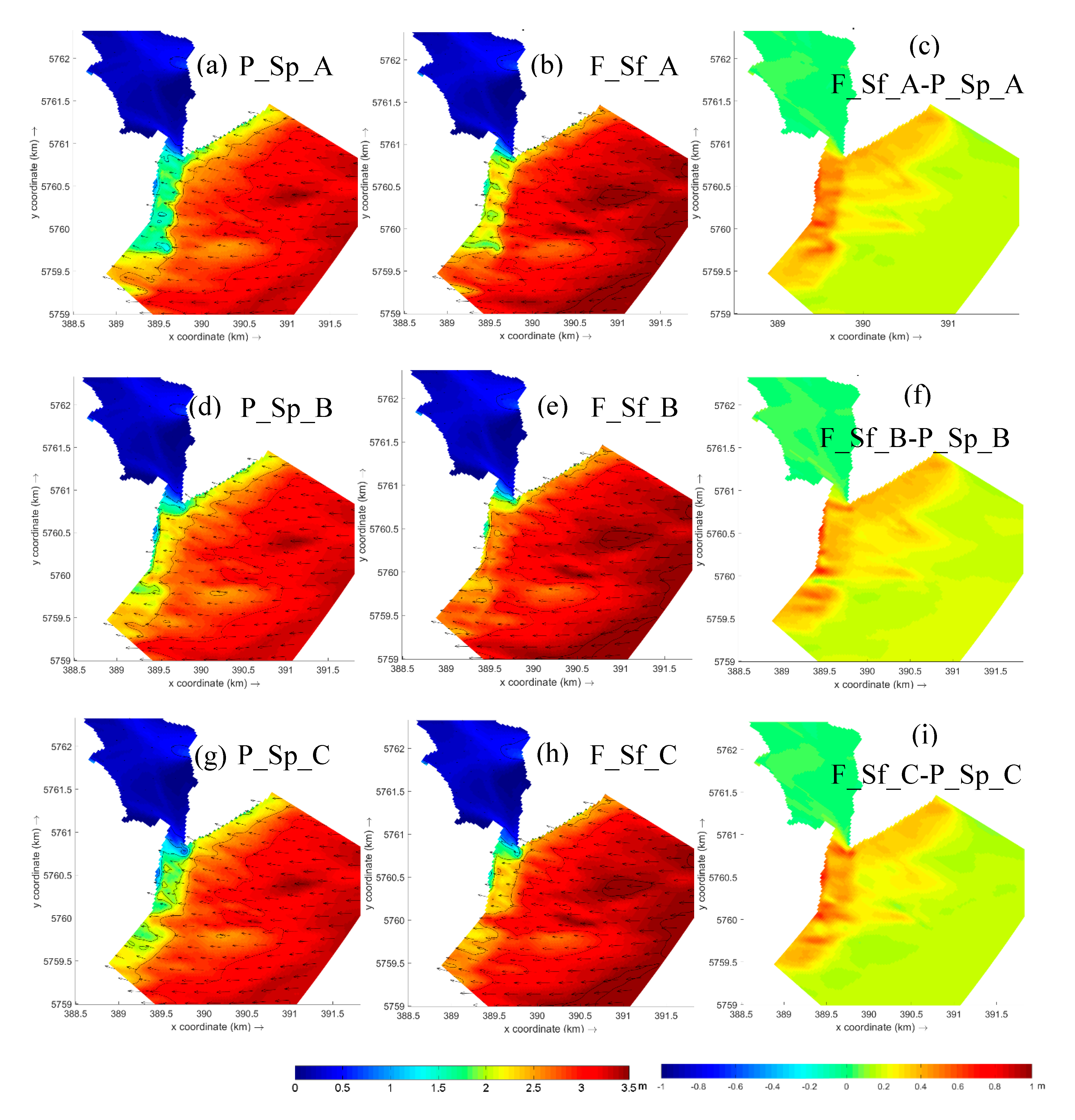
When the estuary is in morphodynamic State A, the ebb shoal is at a fully developed state and the ebb jet has migrated southwards (see the velocities in Figure 16a). The crest of the shoal remains immersed at highest spring tide. The modelled spatial distributions of 1 in 100-year storm wave heights at the storm peak for both ‘present’ and ‘future’ scenarios are shown in Figure 12a,b. In the ‘present’ scenario (Figure 12a), the wave heights reduce significantly when waves approach the inlet due to shallow elongated ebb shoal. The maximum wave height in the inlet and throat areas remain less than 2.0 m. Wave heights in the down-drift and up-drift areas of the inlet remain larger than those at the inlet. It can also be seen that wave heights shoreward of the throat of the inlet remain less than 0.5 m, indicating limited wave penetration into the estuary. In the ‘future’ scenario (Figure 12b), the trend of spatial variability is mostly similar to that under the ‘present’ scenario however, the maximum wave height before the throat area reaches 2.5 m, which is 0.5 m higher than that under the ‘present’ scenario (Figure 12c). Maximum wave height in the down-drift and up-drift areas reached 3.0 m. It should be noted that despite significant differences in storm waves at the inlet and the surroundings under ‘present’ and ‘future’ climates, waves inside the estuary remain largely unchanged. This was mentioned by Burningham et al. [32] that waves in the inner estuary is limited to fetch-limited wind waves as a result of the restricted throat of the estuary which hinders wave penetration from the sea.
It can be seen in Figure 12 (top) that the incoming waves rapidly dissipate at the ebb shoal. The increased future wave height in the inlet area shoreward of the ebb shoal may be partly due to the increased water level due to SLR under ‘future’ scenario.
4.1.2. Morphodynamic Changes
Although we focus only on short term morphodynamic change during storm events in a future climate ‘snap-shot’, potential future changes to the littoral sediment transport regime as a result of higher wave heights and water levels prevailing in the ebb shoal area may have implications on the long-term morphology change of the estuary as reported in [33] which states that morphodynamic life cycle of the inlet and the ebb shoal is strongly linked to the prevailing littoral transport regime.
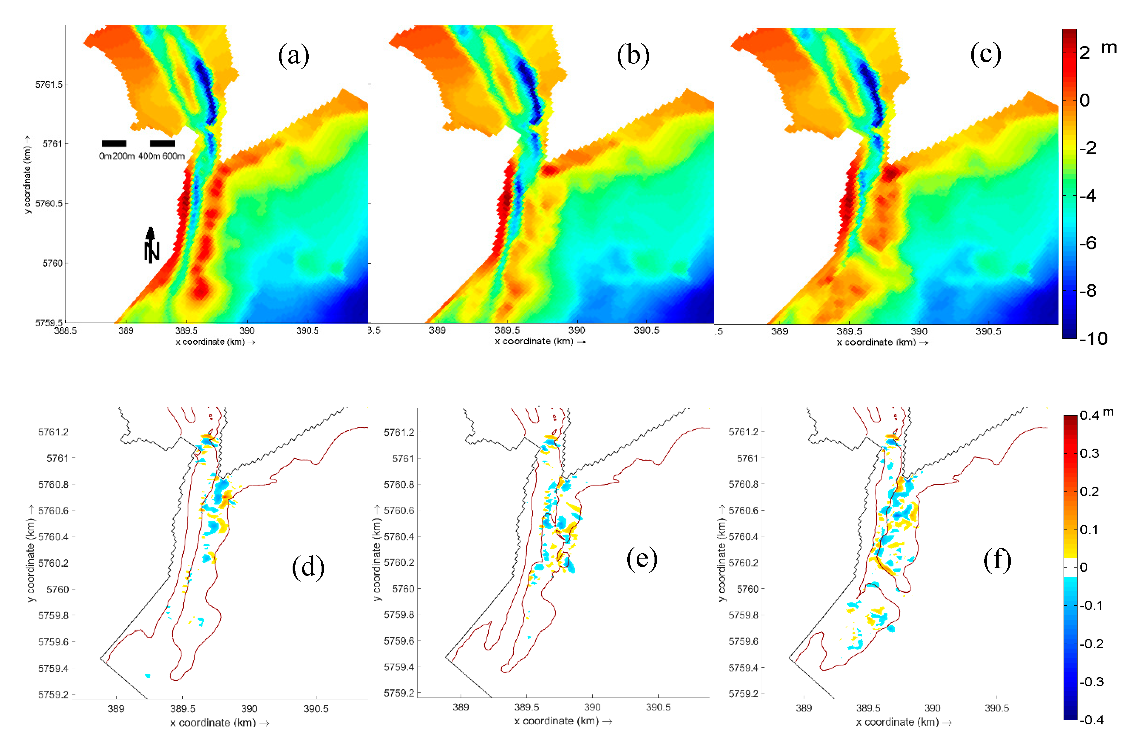
The cumulative morphology changes during the 1 in 100-year ‘present’ and ‘future’ storm scenarios are shown in Figure 13b,c. It can be seen that the cumulative morphological changes under the ‘present’ scenario are most obvious at the throat and the north ebb shoal. Morphology change under the ‘future’ scenario is significantly higher than that under ‘present’ scenario. In addition to throat and north ebb shoal, seabed erosion spreads along the ebb shoal, indicating the potential for a breach. The ebb shoal acts as a wave shield when the estuary is in State A. Therefore, erosion or potential breach of the shoal, thus exposing the coastline into incoming waves and tides, may have notable implications on the morphodynamic characteristics of the estuary onshore in future.
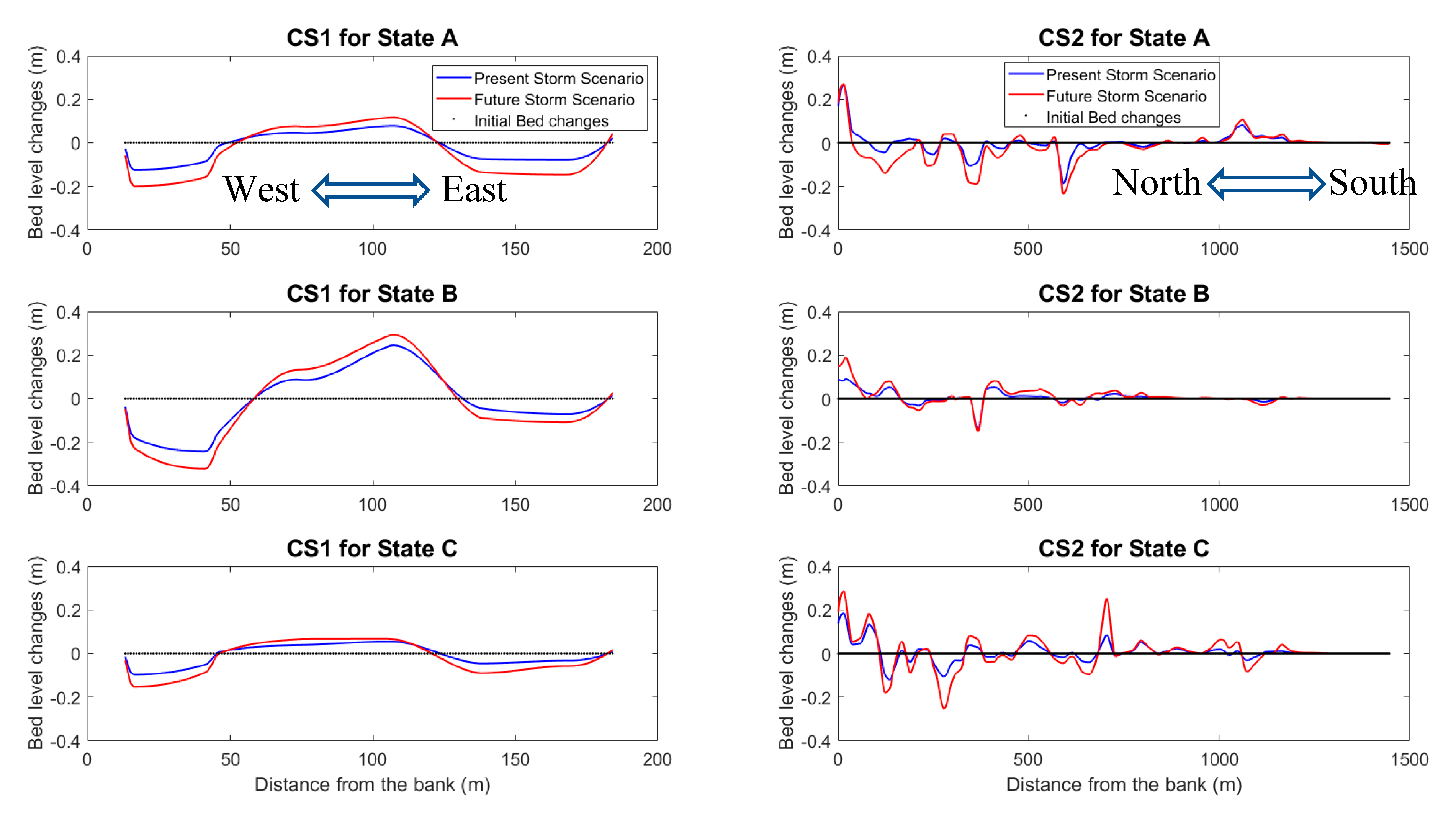
To explore the impacts of storms on the most important morphodynamic elements of the Deben estuary inlet in detail, two cross sections are selected: (i) A section crossing the throat of the inlet (named as ‘CS1′) and, (ii) a section along the crest of the ebb shoal (named as ‘CS2′) (black lines in Figure 13a). The bed level change occurred at these two cross sections during the ‘present’ and ‘future’ 1 in 100-year storms are shown in Figure 14 (top). The increased SLR and storm conditions in the future would increase erosion/deposition rate at both sections without changing the pattern of bed level change. This means the eroded (deposited) locations under ‘present’ storm scenario will be more eroded (deposited) under ‘future’ storm conditions. At cross section ‘CS2′ the ‘future’ 1 in 100-year storm will not only enhance erosion at the north of the shoal crest but will also increase the deposition rate of the south shoal although the changes in the north are more significant (Figure 14). Generally, potential breach of the ebb shoal may be more severe under the ‘future’ storm condition when the inlet is in morphodynamic State A.
4.2. Estuary State B
4.2.1. Waves and Hydrodynamic Changes
When the estuary inlet is in morphodynamic State B, (Figure 11b), where the northern part of the ebb shoal has broken into segments and has become deeper, ebb tidal currents on the ebb shoal spread over a wider region due to the segmented shoal and hence the velocities in the main channel become smaller (see the velocities in Figure 16c).
The spatial distribution of 1 in 100-year storm wave heights at the storm peak under both ‘present’ and ‘future’ scenarios when the estuary is in this state are shown in Figure 12d,e. The figures show that the wave heights under both ‘present’ and ‘future’ scenarios are much larger than that in State A, potentially due to the severely fragmented deeper ebb shoal which allows more wave penetration into the inlet area of estuary. The increased water depth due to SLR in ‘future’ condition allows waves to reach further onshore before breaking thus contributing to increased nearshore wave heights. However, similar to State A, the waves are not able to propagate into the inner estuary due to the restricted throat of the inlet.
4.2.2. Morphodynamic Changes
Cumulative change of State B morphology during the ‘present’ and ‘future’ 1 in 100-year storms are shown in Figure 13e,f. It can be seen that the bed level change in both scenarios are concentrated around the northern part of the ebb shoal while the bed level change is larger and more extensive under the ‘future’ storm scenario. In this case, some notable bed level changes can also be seen at the throat area. The differences of bed level changes at throat areas between ‘present’ and ‘future’ scenarios in both State A and B are similar (Figure 15d,e).
It can be noted that ‘future’ storm not only increases the deposition/erosion rate at the north ebb shoal where deposition occurs predominantly but also makes the ebb shoal more morphodynamically active on average. The inner estuary is not notably affected, similar to State A.
4.3. Estuary State C
4.3.1. Waves and Hydrodynamic Changes
When the estuary is in morphodynamic State C, the ebb shoal is fragmented into two distinct shoals by the development of a primary ebb jet channel towards the south-east side, within which the ebb tide currents are concentrated, (see the velocities in Figure 16e). The spatial distributions of 1 in 100-year storm wave heights at the storm peak in both ‘present’ and ‘future’ scenarios are shown in Figure 12g,h. Both figures show higher wave activities in the ebb jet area. The magnitude of 1 in 100-year storm wave heights on the ebb shoals in this state are between State A and B (Figure 12).
4.3.2. Morphodynamic Changes
Since the entire ebb shoal is segmented by the primary ebb jet channel in State C, the erosion and deposition on the entire ebb shoal become more severe than in State A and State B (Figure 13h) and (Figure 13i). Both north and south ebb shoals experience significant changes under the ‘future’ storm conditions. Apart from the more pronounced erosion/deposition pattern on the south ebb shoal under future scenario, the most notable changes along the ebb shoal crest are the increased erosion of north ebb shoal and increased deposition in ebb jet region (bottom figures in Figure 14). Although the throat of the inlet in this state also becomes dynamic (but less than previous two states), the difference of morphodynamic changes between ‘present’ and ‘future’ scenarios are not significant (Figure 14). In summary it can be observed that the ebb shoal in State C is the most morphodynamically vulnerable while the throat area is not dynamic compared to the other two states.
4.4. Cross-Comparisons among the Different Estuary Morphodynamic States
Cross-comparisons of morphodynamic response of the Deben Estuary inlet to present and future 1 in 100-year storm when the inlet is in morphodynamic states of A, B, and C are shown in Figure 15. Two common features can be noted: (i) The northern part of the ebb shoal area is likely to undergo significant changes under future extreme conditions, irrespective of the prevailing morphodynamic state; and (ii) the inner estuary undergoes negligible changes. However, the difference of bed level changes between ‘future’ and ‘present’ storm scenarios also illustrates the variations of the morphodynamic responses to the change in storm climate among the three selected states. More specifically, the most morphodynamically responsive area to future storms when the inlet is at State A and B remains to be the northern part of the ebb shoal, although the covered dynamic area in State B is slightly more extensive in cross-shore direction than that in State A. In State C, the entire ebb shoal becomes more dynamic under future storm conditions whereas the changes of ebb jet region will not be modified too much by the future storms. The throat of the inlet in all morphodynamic states show a pattern of erosion in the offshore side and accretion in the onshore side under the storm conditions among which the throat cross changes in State B are observed to be the most significant. It can be noted that future storm conditions exacerbate erosion and deposition of the throat area in all states by similar amounts (Figure 14). This can be attributed to the similar tidal currents passing through the throat and limited change of wave heights reaching to the inlet in all morphodynamic states between ‘present’ and ‘future’ scenarios.
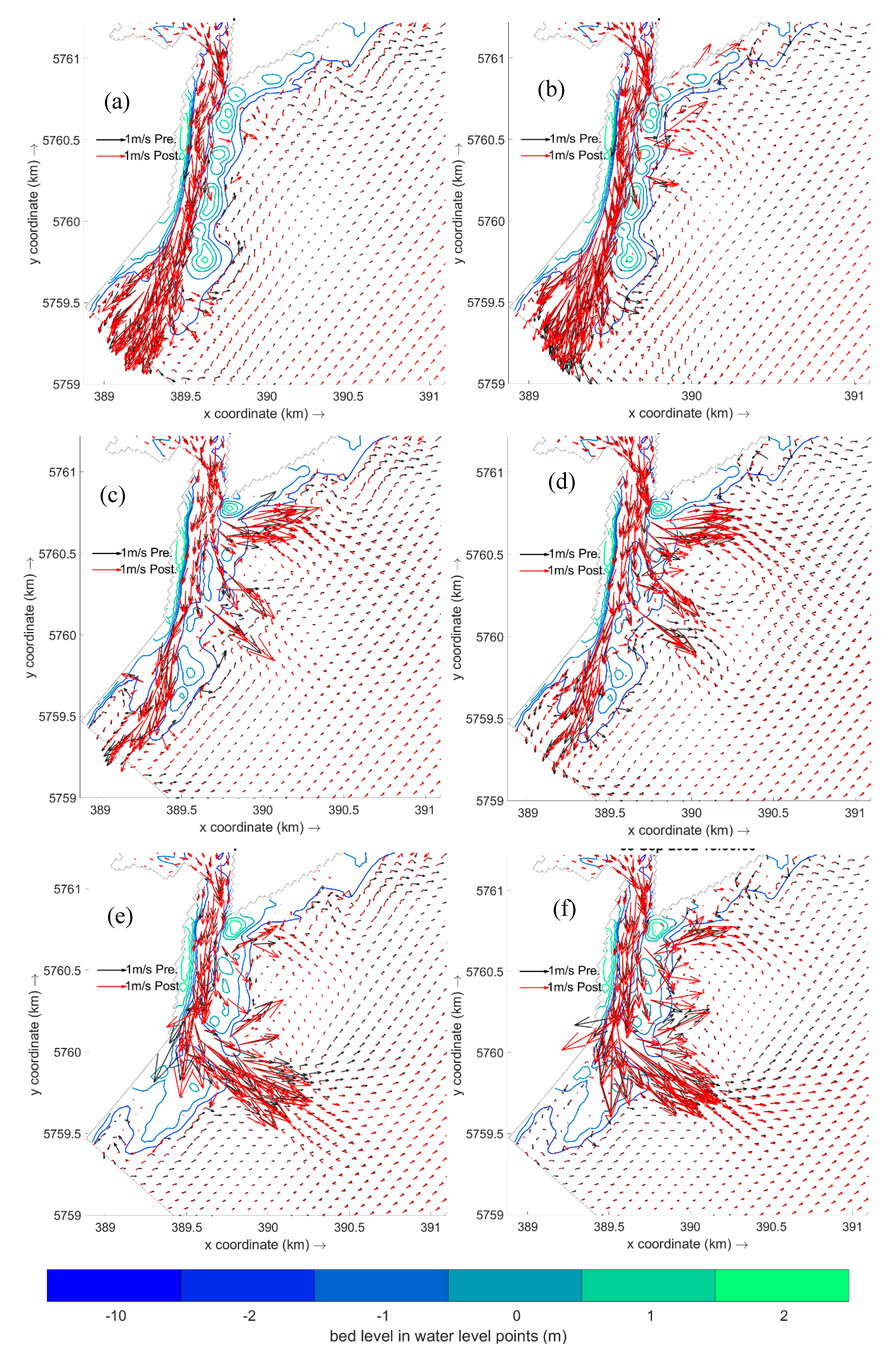
Although morphodynamic change of the estuary inlet from one storm may not be detrimental to the stability and integrity of the inlet, perturbations induced by the storms on the morphodynamically vulnerable ebb shoal area may adversely impact the nature and the frequency of the prevailing cyclic morphodynamic evolution trend of the inlet or may deviate the inlet from the current trend of evolution altogether. For example, in State C, enhancement of the second ebb jet in the northern side of the shoal (Figure 16e,f), and hence the passage of stronger tidal currents may positively contribute to further fragmentation and destabilization of the shoal thus reducing its ability to recover and hence the ability to maintain the cyclic evolution pattern.
A snapshot of the differences in ebb tidal currents (strongest during a tidal cycle, which is important in ebb-dominated estuary) under spring tides in and around the inlet before and after the storm are seen in Figure 16. For State A, post-storm ebb currents in the north ebb shoal area are significantly higher than that of pre-storm ebb currents for both present and future storm scenarios. Post-storm ebb currents in the south shoal area are not notably different from its pre-storm values for both present and future conditions, which agrees well with less morphology change in the south shoal area (Figure 15d). In State B, post-storm tidal currents all throughout the shoal under both present and future storm scenarios are notably different from the pre-storm currents where stronger currents are observed in the eroded north-east areas of the shoal. In State C, unlike in State A and B, the strongest ebb currents can be seen towards south-east direction under both present and future storms. However, most notable changes to the post-storm currents can be seen in the north shoal area and the changes observed under future storm scenario is notably stronger than that observed under present storm scenario.
The differences between pre- and post-storm tidal currents under both present and future storm conditions can be attributed to two factors: (i) Morphodynamic change during the storm; and (ii) higher water level during the ‘future’ storm as a result of SLR and hence the reduction in inter-tidal areas. It should be noted that the intertidal areas during the astronomic spring tides in State A, State B, and State C are reduced by 18.9%, 28.9%, and 15.9%, respectively as a result of SLR, where State B has undergone the largest reduction.
5. Conclusions
The morphodynamic response of a meso-tidal Deben Estuary inlet to future changes of extreme storm conditions and sea level was investigated using a process-based numerical model. The model was extensively validated against measured wave, tide, and bathymetry change data prior to applying it for investigating the storm impacts on the inlet.
As the Deben Estuary evolves through natural morphodynamic cycles under the prevailing wave and tide regimes, the estuary currently goes through three predominant morphodynamic states A, B, and C where the inlet of the estuary goes through a substantial morphodynamic transformation. Although in State C, the ebb shoal of the estuary undergoes fragmentation, the estuary currently has the ability to revive over a certain period of time and repair the shoal thus eventually transforming it back into State A with a fully developed shoal. This process sustains on the delicate balance between the prevailing hydrodynamic and sediment transport regimes. Any perturbations to this as a result of future climate change can potentially change this cycle, which was investigated in this study.
As Deben is a meso-tidal estuary with large intertidal areas, one would expect the estuary may not be notably sensitive to a slight increase in storm conditions. However, our modelling results show otherwise where the inlet can be adversely affected by storms where the most morphodynamically active ebb shoal can undergo rapid morphodynamic changes during storms. Although the severity and frequency of storms and surges in the North Sea, where the estuary is located, have found to increase only marginally as a result of global climate change, future storms combined with the increased sea levels found to have notable impacts on the morphodynamic behavior of the inlet. It was also found that implication of extreme storm attacks, if occurred when the estuary is in the morphodynamic State C, will be more severe than that they occurred when the estuary is in States A or B, associated with the tide and SLR effects.
The results of this 2D model study show potential implications of storm-induced changes on the morphodynamics of the Deben Estuary inlet. These findings are important to interpret the behavior of the Deben Estuary in the long-term [27]. The results clearly show that future storms and sea level rise may contribute to destabilize the current cyclic morphodynamic regime of the estuary, which will have significant consequences on the estuary itself and the surrounding shorelines as the estuary is strongly morphodynamically linked with the surrounding coastlines [27].
Some limitations of our modelling approach should be noted. Although estuary bathymetry may gradually accommodate to future sea level variations, we used historically available measured bathymetries for modelling future storm impacts, as a better alternative was not available. Simulating bathymetry change using a process-based model for 100 years is unrealistic, unreliable, and not feasible due to uncertainties and accumulation of numerical errors. Therefore, the ‘snap-shot’ approach we used here, which has been successfully used by other researchers to investigate climate change impacts on estuaries (e.g., [27,28,29]), is only the best way to achieve the aims of this study. Additionally, we limited ourselves to 1 in 100-year storms, with the worst-case scenario of storm peak coinciding with highest tide and peak surge. We may assume that storm events with less severity will induce less severe morphodynamic changes. Although we consider only one future climate scenario, it will be useful to investigate morphodynamic change under a range of future climate scenarios to assess the uncertainties associated with future climate change, for example, using the ensemble methods [13,52].
Although our research focused on one estuary, the models and methods used are easily transferable to any estuary systems. Moreover, the results of this study give a clear insight into how alterations of different dynamic forcing resulted from climate change contribute to estuarine morphodynamics. The findings of this research can provide references for coastal and estuarine managers when taking management decisions and developing intervention scenarios for sustainable estuary management in future.
Author Contributions
Conceptualization, Y.Y. and H.K.; Methodology, Y.Y. and H.K.; Data analysis, Y.Y.; Investigation, Y.Y.; Writing—original draft preparation, Y.Y.; Writing—review and editing, H.K. and D.E.R.; Supervision, H.K. and D.E.R.
Acknowledgments
The authors acknowledge the UK Natural Environment Research Council (NERC) funded iCOASST (NE/J005606/1) project for providing the bathymetry data of the Deben Estuary, British Oceanography Data Centre (BODC) and CEFAS for providing tide and wave data, respectively. We also acknowledge Nobuhito Mori at the Disaster Prevention Research Institute of Kyoto University for providing projected current and future wave data from Japanese Meteorological Research Institute and the Japan Meteorological Agency (MRI-JMA). The first author acknowledges the China Scholarship Council (CSC) and the College of Engineering of Swansea University for jointly funding his PhD studies at Swansea University, UK.
Conflicts of Interest
The authors declare no conflict of interest.
References
- Bruun, P. Sea-level rise as a cause of shore erosion. J. Waterw. Harb. Div. 1962, 88, 117–130. [Google Scholar]
- Gornitz, V.; Couch, S.; Hartig, E.K. Impacts of sea level rise in the New York City metropolitan area. Glob. Planet. Chang. 2001, 32, 61–88. [Google Scholar] [CrossRef]
- Stive, M. How important is global warming for coastal erosion? Clim. Chang. 2004, 64, 27–39. [Google Scholar] [CrossRef]
- Van Goor, M.A.; Zitman, T.J.; Wang, Z.B.; Stive, M.J.F. Impact of sea-level rise on the morphological equilibrium state of tidal inlets. Mar. Geol. 2003, 202, 211–227. [Google Scholar] [CrossRef]
- Van Der Wal, D.; Pye, K.; Neal, A. Long-term morphological change in the Ribble Estuary, northwest England. Mar. Geol. 2002, 189, 249–266. [Google Scholar] [CrossRef]
- Long, A.J.; Innes, J.B.; Lloyd, J.M.; Rutherford, M.M.; Shennan, I.; Kirby, J.R.; Tooley, M.J. Holocene sea-level change and coastal evolution in the Humber estuary, eastern England: An assessment of rapid coastal change. Holocene 1998, 8, 229–247. [Google Scholar] [CrossRef]
- Guthrie, G.; Cottle, R. Suffolk Coast and Estuaries Coastal Habitat Management Plan; Report to English Nature/Environment Agency; Posford Haskoning Ltd.: Peterborough, UK, 2002; Appendix A; pp. 20–25. [Google Scholar]
- Horrillo-Caraballo, J.M.; Reeve, D.E.; Simmonds, D.; Pan, S.; Fox, A.; Thompson, R.; Hoggarth, S.; Kwan, S.S.H.; Greaves, D. Application of a source-pathway-receptor-consequence (S-P-R-C) methodology to the Teign Estuary, UK. J. Coast. Res. Spec. Issue 65 Int. Coast. Symp. 2013, 2, 1939–1944. [Google Scholar] [CrossRef]
- Tessier, B.; Billeaud, I.; Sorrel, P.; Delsinne, N.; Lesueur, P. Infilling stratigraphy of macrotidal tide-dominated estuaries. Controlling mechanisms: Sea-level fluctuations, bedrock morphology, sediment supply and climate changes (The examples of the Seine estuary and the Mont-Saint-Michel Bay, English Channel, NW France). Sediment. Geol. 2012, 279, 62–73. [Google Scholar] [CrossRef]
- Robins, P.E.; Skov, M.W.; Lewis, M.J.; Giménez, L.; Davies, A.G.; Malham, S.K.; Neill, S.P.; McDonald, J.E.; Whitton, T.A.; Jackson, S.E.; et al. Impact of climate change on UK estuaries: A review of past trends and potential projections. Estuar. Coast. Shelf Sci. 2016, 169, 119–135. [Google Scholar] [CrossRef]
- Houghton, G.T.; Ding, Y.; Griggs, D.J.; Noguer, M.; Van der Linden, P.J.; Dai, X.; Maskell, K.; Johnson, C.A. Climate Change Scientific Basis, Contribution of Working Group 1 to the Third Assessment Report of the Intergovernmental Panel on Climate Change (IPCC); Cambridge University Press: Cambridge, UK, 2001; pp. 74–77. [Google Scholar]
- Lowe, J.A.; Howard, T.P.; Pardaens, A.; Tinker, J.; Holt, J.; Wakelin, S.; Milne, G.; Leake, J.; Wolf, J.; Horsburgh, K.; et al. UK Climate Projections Science Report: Marine and Coastal Projections; Met Office Hadley Centre: Exeter, UK, 2009. [Google Scholar]
- Woth, K.; Weisse, R.; Von Storch, H. Climate change and North Sea storm surge extremes: An ensemble study of storm surge extremes expected in a changed climate projected by four different regional climate models. Ocean Dyn. 2006, 56, 3–15. [Google Scholar] [CrossRef]
- Jenkins, G.J.; Murphy, J.M.; Sexton, D.M.H.; Lowe, J.A.; Jones, P.; Kilsby, C.G. UK Climate Projections: Briefing Report; Met Office Hadley Centre: Exeter, UK, 2009. [Google Scholar]
- Meehl, G.A.; Stocker, T.F.; Collins, W.; Friedlingstein, P.; Gaye, A.; Gregory, J.; Kitoh, A.; Knutti, R. Global climate projections. In Climate Change 2007: The Physical Science Basis. Contribution of Working Group I to the Fourth Assessment Report of the Intergovernmental Panel on Climate Change; Solomon, S., Qin, D., Manning, M., Chen, Z., Marquis, M., Averyt, K.B., Tignor, M., Miller, H.L., Eds.; Cambridge University Press: Cambridge, UK, 2007; pp. 747–846. [Google Scholar]
- Nicholls, R.J.; Wong, P.P.; Burkett, V.R.; Codignotto, J.O.; Hay, J.E.; McLean, R.F.; Ragoonaden, S.; Woodroffe, C.D. Coastal systems and low-lying areas. In Climate Change 2007: Impacts, Adaptation and Vulnerability. Contribution of Working Group II to the Fourth Assessment Report of the Intergovernmental Panel on Climate Change; Parry, M.L., Canziani, O.F., Palutikof, J.P., van der Linden, P.J., Hanson, C.E., Eds.; Cambridge University Press: Cambridge, UK, 2007; pp. 315–356. [Google Scholar]
- Brown, J.M.; Wolf, J. Coupled wave and surge modelling for the eastern Irish Sea and implications for model wind-stress. Cont. Shelf Res. 2009, 29, 1329–1342. [Google Scholar] [CrossRef]
- Brown, J.M.; Souza, A.J.; Wolf, J. Surge modelling in the eastern Irish Sea: Present and future storm impact. Ocean Dyn. 2010, 60, 227–236. [Google Scholar] [CrossRef]
- Chini, N.; Stansby, P.; Leake, J.; Wolf, J.; Roberts-Jones, J.; Lowe, J. The impact of sea level rise and climate change on inshore wave climate: A case study for East Anglia (UK). Coast. Eng. 2010, 57, 973–984. [Google Scholar] [CrossRef]
- Wang, X.; Swail, V.R. Trends of Atlantic Wave Extremes as Simulated in a 40-Yr Wave Hindcast Using Kinematically Reanalyzed Wind Fields. J. Clim. 2001, 15, 1020–1035. [Google Scholar] [CrossRef]
- Wolf, J.; Brown, J.M.; Howarth, M.J. The wave climate of Liverpool Bay-observations and modelling. Ocean Dyn. 2011, 61, 639–655. [Google Scholar] [CrossRef]
- Brown, J.M.; Wolf, J.; Souza, A.J. Past to future extreme events in Liverpool Bay: Model projections from 1960–2100. Clim. Chang. 2012, 111, 365–391. [Google Scholar] [CrossRef]
- Dissanayake, D.M.P.K.; Ranasinghe, R.; Roelvink, J.A. Effects of sea level rise in tidal inlet evolution: A numerical modelling approach. J. Coast. Res. 2009, 11, 942–946. [Google Scholar]
- Lesser, G.; Roelvink, J.; van Kester, J.; Stelling, G. Development and validation of a three-dimensional morphological model. Coast. Eng. 2004, 51, 883–915. [Google Scholar] [CrossRef]
- Karunarathna, H.; Reeve, D.E. A Boolean approach to prediction of long-term evolution of estuary morphology. J. Coast. Res. 2008, 24, 51–61. [Google Scholar] [CrossRef]
- Passeri, D.L.; Hagen, S.C.; Medeiros, S.C.; Bilskie, M.V. Impacts of historic morphology and sea level rise on tidal hydrodynamics in a microtidal estuary (Grand Bay, Mississippi). Cont. Shelf Res. 2015, 111, 150–158. [Google Scholar] [CrossRef]
- Yin, Y.; Karunarathna, H.; Reeve, D.E. Numerical modelling of hydrodynamic and morphodynamic response of a meso-tidal estuary inlet to the impacts of global climate variabilities. Mar. Geol. 2019, 407, 229–247. [Google Scholar] [CrossRef]
- Duong, T.M.; Ranasinghe, R.; Luijendijk, A.; Walstra, D. Assessing climate change impacts on the stability of small tidal inlets: Part 1-Data poor environments. Mar. Geol. 2017, 390, 331–346. [Google Scholar] [CrossRef]
- Duong, T.M.; Ranasinghe, R.; Thatcher, M.; Mahanama, S.; Wang, Z.B.; Dissanayake, P.K.; Hemer, M.; Luijendijk, A.; Bamunawala, J.; Roelvink, D.; et al. Assessing climate change impacts on the stability of small tidal inlets: Part 2-Data rich environments. Mar. Geol. 2018, 395, 65–81. [Google Scholar] [CrossRef] [PubMed]
- ABPmer. Development and Demonstration of Systems-Based Estuary Simulators. R&D Technical Report FD2117/TR; Department for Environment, Food and Rural Affairs (DEFRA): London, UK, March 2008. [Google Scholar]
- Beardall, C.H.; Dryden, R.C.; Holzer, T.J. The Suffolk Estuaries; Segment Publications: Colchester, UK, 1991; p. 77. [Google Scholar]
- Burningham, H.; French, J. Morphodynamic behaviour of a mixed sand–gravel ebb-tidal delta: Deben estuary, Suffolk, UK. Mar. Geol. 2006, 225, 23–44. [Google Scholar] [CrossRef]
- HR Wallingford; CEFAS; Posford Haskoning; D’Olier, B. Southern North Sea Sediment Transport Study (Phase 2); Report EX; HR Wallingford Ltd: Wallingford, UK, 2002. [Google Scholar]
- Hydrographic Office. Admiralty Tide Tables: United Kingdom and Ireland (Including European Channel Ports); Hydrographer of the Navy: Taunton, UK, 2000; p. 440. [Google Scholar]
- Posford Duvivier. Suffolk Estuarine Strategies: Deben Estuary. Strategy Report: Phase 2 Volume 1 Main Report; Environment Agency: Peterborough, UK, 1999; pp. 5–20. [Google Scholar]
- Wong, P.P.; Losada, I.J.; Gattuso, J.-P.; Hinkel, J.; Khattabi, A.; McInnes, K.L.; Saito, Y.; Sallenger, A. Coastal systems and low-lying areas. In Climate Change 2014: Impacts, Adaptation, and Vulnerability. Part A: Global and Sectoral Aspects. Contribution of Working Group II to the Fifth Assessment Report of the Intergovernmental Panel on Climate Change; Field, C.B., Barros, V.R., Dokken, D.J., Mach, K.J., Mastrandrea, M.D., Bilir, T.E., Chatterjee, M., Ebi, K.L., Estrada, Y.O., Genova, R.C., et al., Eds.; Cambridge University Press: Cambridge, UK; New York, NY, USA, 2014; pp. 361–409. [Google Scholar]
- Solomon, S.; Quin, D.; Manning, M.; Chen, Z.; Marquis, M.; Averyt, K.; Tignor, M.; Miller, H.L., Jr. (Eds.) Climate Change 2007: The Physical Science Basis; Cambridge University Press: Cambridge, UK, 2007; p. 996. [Google Scholar]
- Mizuta, R.; Yoshimura, H.; Endo, H.; Ose, T.; Kamiguchi, K.; Hosaka, M.; Sugi, M.; Yukimoto, S.; Kusunoki, S.; Kitoh, A. Climate Simulations Using MRI-AGCM3.2 with 20-km Grid. J. Meteorol. Soc. Jpn. 2012, 90, 233–258. [Google Scholar] [CrossRef]
- Shimura, T.; Mori, N.; Mase, H. Future projection of ocean wave climate: Analysis of SST impacts on wave climate changes in the Western North Pacific. J. Clim. 2015, 18, 3171–3190. [Google Scholar] [CrossRef]
- Tolman, H.L. User Manual and System Documentation of WAVEWATCH-III; TM Version 3.14; Technical note; U.S. Department of Commerce NOAA, National Centers for Environmental Prediction: Camp Springs, MD, USA, May 2009. [Google Scholar]
- Murakami, H.; Wang, Y.; Sugi, M.; Yoshimura, H.; Mizuta, R.; Shindo, E.; Adachi, Y.; Yukimoto, S.; Hosaka, M.; Kitoh, A.; et al. Future changes in tropical cyclone activity projected by the new high-resolution MRI-AGCM. J. Clim. 2012, 25, 3237–3260. [Google Scholar] [CrossRef]
- Bennett, W.G.; Karunarathna, H.; Mori, N.; Reeve, D.E. Climate change impacts on future wave climate around the UK. J. Mar. Sci. Eng. 2016, 4, 78. [Google Scholar] [CrossRef]
- Dissanayake, P.; Brown, J.; Wisse, P.; Karunarathna, H. Comparison of storm cluster vs isolated event impacts on beach/dune morphodynamics. Estuar. Coast. Shelf Sci. 2015, 164, 301–312. [Google Scholar] [CrossRef]
- Coles, S. An Introduction to Statistical Modeling of Extreme Values; Springer Series in Statistics: Bristol, UK, 2001. [Google Scholar] [CrossRef]
- Davison, A.C. Modelling excesses over high thresholds, with an application. In Statistical Extremes and Applications; Tiago de Oliveira, J., Ed.; D. Reidel Publishing Company: Dordrecht, The Netherlands, 1984; pp. 461–482. [Google Scholar]
- Booij, N.; Ris, R.; Holthuijsen, L. A third-generation wave model for coastal regions, Part I, Model description and validation. J. Geophys. Res. 1999, 104, 7649–7666. [Google Scholar] [CrossRef]
- Bijker, E. Longshore transport computation. ASCE J. Waterw. Port Coast. Ocean Eng. 1971, 97, 687–701. [Google Scholar]
- Yin, Y. Morphodynamic Responses of Estuaries to Climate Change. Ph.D. Thesis, Swansea University, Swansea, UK, 2018. [Google Scholar]
- Mangor, K.; Drønen, N.K.; Kaergaard, K.H.; Kristensen, N.E. Shoreline Management Guidelines; DHI: Hirschholm, Denmark, 2017. [Google Scholar]
- Battjes, J.; Janssen, J. Energy loss and set-up due to breaking of random waves. In No 16 (1978): Proceedings of 16th Conference on Coastal Engineering, Hamburg, Germany, 1978; ASCE: Reston, VA, USA, 1978; pp. 569–587. [Google Scholar]
- McMillan, A.; Batstone, C.; Worth, D.; Tawn, J.; Horsburgh, K.; Lawless, D. Coastal Flood Boundary Conditions for UK Mainland and Islands; Technical report; Environment Agency/Defra: Bristol, UK, 2011. [Google Scholar]
- Zou, Q.P.; Chen, Y.; Cluckie, I.; Hewston, R.; Pan, S.; Peng, Z.; Reeve, D. Ensemble prediction of coastal flood risk arising from overtopping by linking meteorological, ocean, coastal and surf zone models. Q. J. R. Meteorol. Soc. 2013, 139, 298–313. [Google Scholar] [CrossRef]
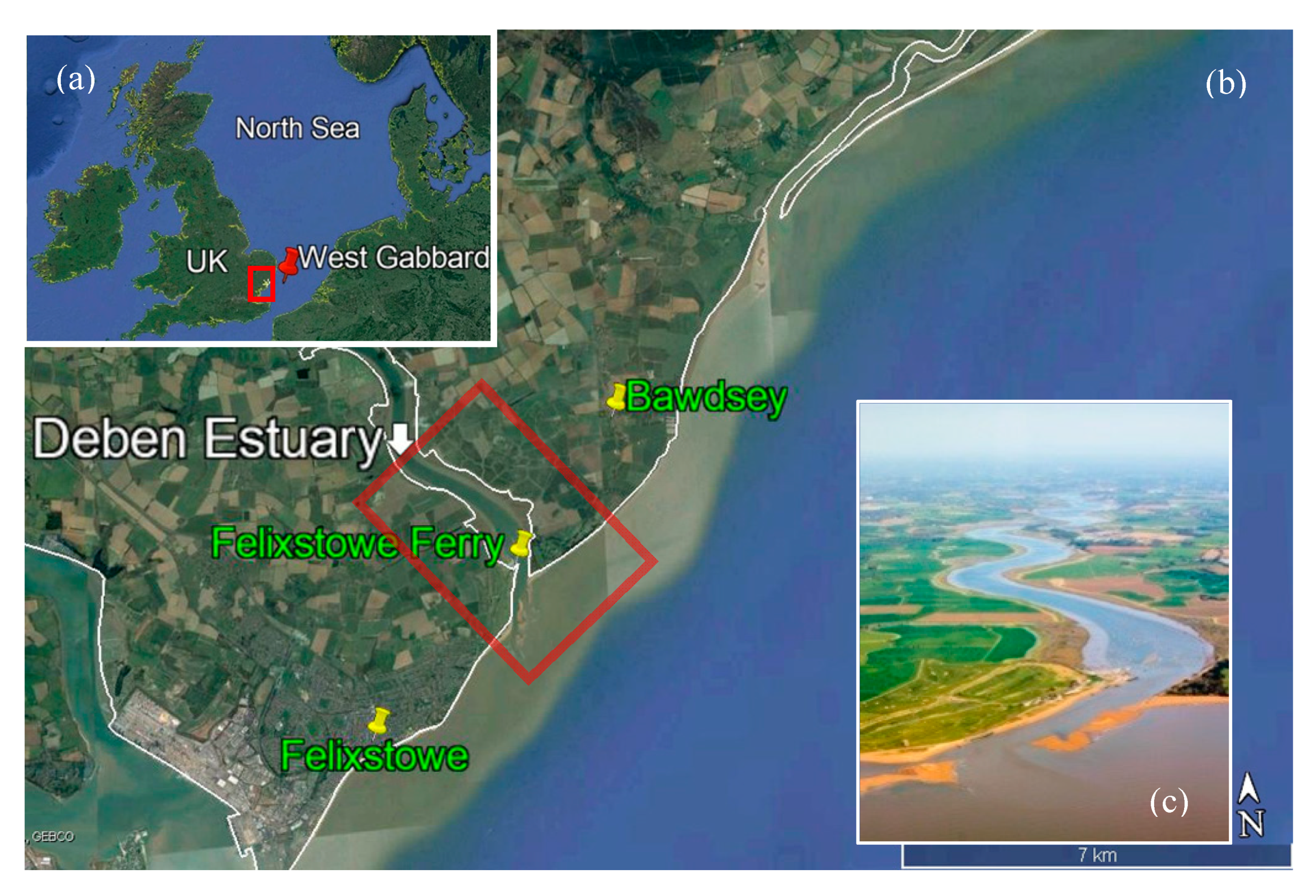
Figure 1.
The location of Deben Estuary in the UK (the red square in (a)), Deben surroundings (b) [extracted from Google maps] and close view of the inlet area of estuary (c) [photo from website of River Deben Association: riverdeben.org]. The wave buoy ‘West Gabbard’ is shown by the red marker in (a). The estuary inlet is marked in red square in (b).

Figure 2.
The Relative Sea Level Rise (RSLR) over the 21st century based on three emission scenarios with central estimate values (thick lines) and 5th and 95th percentile limits of the range of uncertainty (thin line) at four sample locations around the UK: London (a), Cardiff (b), Edinburgh (c), Belfast (d). The ‘London’ site (a) is the nearest from Deben Estuary [14]. Figures are adapted with permission from UK Climate Projection 2009 under Open Government License v3.0.

Figure 3.
The global WAVEWATCH Ш model (a) and the nodes around UK area (b) (refer to [42], with permissions from Bennett et al, 2016). The node number stands for the nodes in the global wave model. We use the wave outputs at node 19 (red circle in figure b).
Figure 3.
The global WAVEWATCH Ш model (a) and the nodes around UK area (b) (refer to [42], with permissions from Bennett et al, 2016). The node number stands for the nodes in the global wave model. We use the wave outputs at node 19 (red circle in figure b).

Figure 4.
The comparison of Hs Probability Distribution Function (PDF) (a) and Cumulative Distribution Function (CDF) (b) between modelled (red lines) and measured waves at ‘West Gabbard’ WaveNet site (WGW) (blue lines) and the comparisons of Tp PDF (c) and CDF (d) between modelled (red lines) and measured waves at WGW (blue lines). In order to show bigger values of Hs, the x-coordinate of Hs is scaled by logarithm.

Figure 5.
Empirical quantile–quantile plot of Hs between measured wave data and modelled data.

Figure 6.
The wave roses of observed data (a) and modelled data (b). The color bar indicates the value range of Hs.
Figure 6.
The wave roses of observed data (a) and modelled data (b). The color bar indicates the value range of Hs.

Figure 7.
Storm event definition method (following Bennett et al. [42]). D—duration of storm; IN—interval between two storms; Hs,p—peak storm wave height; Hs Threshold —pre-defined storm threshold; RT — consecutive storm event.
Figure 7.
Storm event definition method (following Bennett et al. [42]). D—duration of storm; IN—interval between two storms; Hs,p—peak storm wave height; Hs Threshold —pre-defined storm threshold; RT — consecutive storm event.

Figure 8.
The mean residual life plot with 95% confidence interval based on ‘present’ Hsmax storm events for the purpose of choosing the storm threshold of GPD (a). Scale (b) and shape (c) parameter estimates against the thresholds for threshold choice revisited purpose.
Figure 8.
The mean residual life plot with 95% confidence interval based on ‘present’ Hsmax storm events for the purpose of choosing the storm threshold of GPD (a). Scale (b) and shape (c) parameter estimates against the thresholds for threshold choice revisited purpose.

Figure 9.
Nested domains of the Delft3D Deben wave and tidal model and validation points in this study. The rectangular points stand for the tide validation locations and circles are wave validation locations. Detailed descriptions and validations can refer to [27]. Adapted with permission from ELSEVIER, 2019.

Figure 10.
(a) Idealized present and future storm profiles, (b) tide and surge conditions used for model simulation. The worst-case scenario where storm peaks on the highest tide was considered. The surge profile was developed based on the normalized surge curve at Felixstowe, located to the south of Deben Estuary (in Figure 1) (reproduced based on the data was from [51] and TPXO7.2).

Figure 11.
The historically cycled morphodynamic states of Deben Estuary (a): adapted from Burningham et al. [32]); the three representative bathymetry states are used as initial bathymetry states for the numerical model in this study (bottom): State A (b); State B (c); State C (d). (The color bar shows depths referred to current mean sea level) (adapted from Yin et al. [27]). All figures are adapted with permission from ELSEVIER, 2006 and 2019.

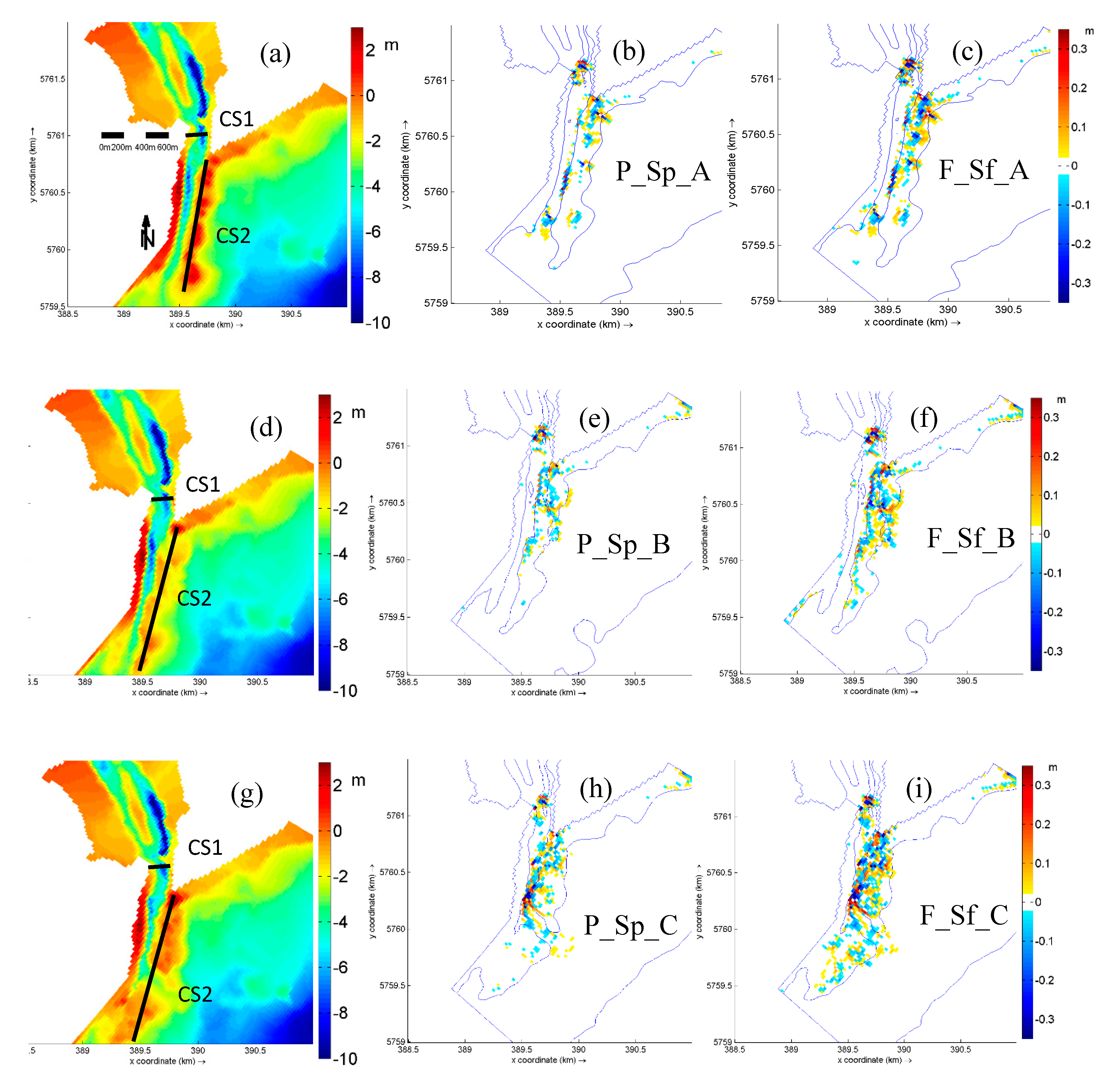
Figure 12.
Storm wave height distributions at and around Deben Estuary under different scenarios (Table 3) in: State A (top), State B (middle), and State C (bottom). (a) Storm wave height distribution under P_Sp_A scenario; (b) Storm wave height distribution under F_Sf_A scenario; (c) difference between F_Sf_A and P_Sp_A (Future minus present); (d) Storm wave height distribution under P_Sp_B scenario; (e) Storm wave height distribution under F_Sf_B scenario; (f) difference between F_Sf_B and P_Sp_B (Future minus present); (g) Storm wave height distribution under P_Sp_C scenario; (h) Storm wave height distribution under F_Sf_C scenario; (i) difference between P_Sf_C and P_Sp_C (Future minus present). The arrows indicate the mean wave directions. All the named scenarios are referred to Table 3.

Figure 13.
The bed level changes under different scenarios (Table 3) based on three different morphological states (Top: State A; Middle: State B; Bottom: State C). (a) initial bathymetry of State A; (b) bed level changes under P_Sp_A scenario; (c) bed level changes under F_Sf_A scenario; (d) initial bathymetry of State B; (e) bed level changes under P_Sp_B scenario; (f) bed level changes under F_Sf_B scenario; (g) initial bathymetry of State C; (h) bed level changes under P_Sp_C scenario; (i) bed level changes under F_Sf_C scenario. The black lines in the left figures are the selected cross sections. All the named scenarios are referred to Table 3.

Figure 14.
The comparison of bed level changes at ‘CS1′ (left) and ‘CS2′ (right) cross sections under ‘present’ and ‘future’ storm scenarios. State A (top), State B (middle), and State C (bottom).
Figure 14.
The comparison of bed level changes at ‘CS1′ (left) and ‘CS2′ (right) cross sections under ‘present’ and ‘future’ storm scenarios. State A (top), State B (middle), and State C (bottom).

Figure 15.
The difference of cumulative erosion and deposition during ‘present’ and ‘future’ scenarios when the estuary is at morphodynamic State A (d), B (e), and C (f) based on the initial bathymetries of State A (a), State B (b) and State C (c). For color bar of the bottom figures: negative values indicate the future bed level change is smaller than the present bed level change; positive values mean the future bed level is larger than present bed level change. The contour line surrounds the shoal area.

Figure 16.
The comparisons of maximum ebb currents between pre-storm (black arrows) and post-storm (red arrows) in every scenario: (a): ‘present’ scenario for State A; (b): ‘future’ scenario for State A; (c): ‘present’ scenario for State B; (d): ‘future’ scenario for State B; (e): ‘present’ scenario for State C; (f): ‘future’ scenario for State C. The color bar stands for the depths and the counter line shows the bathymetry of shoal areas.


Table 1.
Estimated statistically significant peak storm wave heights (Hsmax) with different return periods based on the GPD distributions.
Table 1.
Estimated statistically significant peak storm wave heights (Hsmax) with different return periods based on the GPD distributions.
| Experiments | Estimation Method | 10-year Return Period Hsmax (m) | 20-year Return Period Hsmax (m) | 30-year Return Period Hsmax (m) | 50-year Return Period Hsmax (m) | 100-year Return Period Hsmax (m) | 200-year Return Period Hsmax (m) |
|---|---|---|---|---|---|---|---|
| ‘Present’ | GPD | 5.62 | 5.94 | 6.11 | 6.32 | 6.59 | 6.85 |
| ‘Future’ | GPD | 5.81 | 6.12 | 6.29 | 6.50 | 6.76 | 7.00 |
| Increase from ‘present’ to ‘future’ | GPD | 3.38% | 3.03% | 2.95% | 2.85% | 2.58% | 2.19% |
Table 2.
The Skew Surge Joint Probability Method (SSJPM) results at Felixstowe (values are from [51], adapted with permission from Environment Agency under Open Government License v3.0).
Table 2.
The Skew Surge Joint Probability Method (SSJPM) results at Felixstowe (values are from [51], adapted with permission from Environment Agency under Open Government License v3.0).
| Return Year (years) | 10 | 20 | 25 | 50 | 75 | 100 | 150 | 200 |
|---|---|---|---|---|---|---|---|---|
| Peak Sea Level with 5% confidence interval (mOD) | 3.14 ± 0.2 | 3.29 ± 0.2 | 3.34 ± 0.2 | 3.51 ± 0.2 | 3.62 ± 0.2 | 3.69 ± 0.3 | 3.8 ± 0.3 | 3.88 ± 0.3 |
Table 3.
Modelling scenarios used in this study during the spring tide surge conditions.
| Scenarios | State A-1 in 100-year Storm | State B-1 in 100-year Storm | State C-1 in 100-year Storm |
|---|---|---|---|
| Present | P_Sp_A | P_Sp_B | P_Sp_C |
| Future | F_Sf_A | F_Sf_B | F_Sf_C |
P—Present; F—Future; Sp—Spring tide + present storm; Sf—Spring tide + future storm + SLR: A—State A; B—State B; C—State C.
© 2019 by the authors. Licensee MDPI, Basel, Switzerland. This article is an open access article distributed under the terms and conditions of the Creative Commons Attribution (CC BY) license (http://creativecommons.org/licenses/by/4.0/).
Share and Cite
MDPI and ACS Style
Yin, Y.; Karunarathna, H.; Reeve, D.E. A Computational Investigation of Storm Impacts on Estuary Morphodynamics. J. Mar. Sci. Eng. 2019, 7, 421. https://doi.org/10.3390/jmse7120421
AMA Style
Yin Y, Karunarathna H, Reeve DE. A Computational Investigation of Storm Impacts on Estuary Morphodynamics. Journal of Marine Science and Engineering. 2019; 7(12):421. https://doi.org/10.3390/jmse7120421
Chicago/Turabian StyleYin, Yunzhu, Harshinie Karunarathna, and Dominic E. Reeve. 2019. "A Computational Investigation of Storm Impacts on Estuary Morphodynamics" Journal of Marine Science and Engineering 7, no. 12: 421. https://doi.org/10.3390/jmse7120421
Note that from the first issue of 2016, this journal uses article numbers instead of page numbers. See further details here.