
Deep Collaborative Learning for Randomly Wired Neural Networks


1
Department of Computer Science, Swansea University, Swansea SA1 8EN, UK
2
Department of Computer Science, Faculty of Computers and Information, Mansoura University, Mansoura 35516, Egypt
*
Author to whom correspondence should be addressed.
Electronics 2021, 10(14), 1669; https://doi.org/10.3390/electronics10141669
Submission received: 16 June 2021
/
Revised: 1 July 2021
/
Accepted: 8 July 2021
/
Published: 13 July 2021
(This article belongs to the Section Artificial Intelligence)
Abstract
:A deep collaborative learning approach is introduced in which a chain of randomly wired neural networks is trained simultaneously to improve the overall generalization and form a strong ensemble model. The proposed method takes advantage of functional-preserving transfer learning and knowledge distillation to produce an ensemble model. Knowledge distillation is an effective learning scheme for improving the performance of small neural networks by using the knowledge learned by teacher networks. Most of the previous methods learn from one or more teachers but not in a collaborative way. In this paper, we created a chain of randomly wired neural networks based on a random graph algorithm and collaboratively trained the models using functional-preserving transfer learning, so that the small network in the chain could learn from the largest one simultaneously. The training method applies knowledge distillation between randomly wired models, where each model is considered as a teacher to the next model in the chain. The decision of multiple chains of models can be combined to produce a robust ensemble model. The proposed method is evaluated on CIFAR-10, CIFAR-100, and TinyImageNet. The experimental results show that the collaborative training significantly improved the generalization of each model, which allowed for obtaining a small model that can mimic the performance of a large model and produce a more robust ensemble approach.
1. Introduction
Deep learning has shown powerful performance on many computer vision tasks, such as object recognition [1,2,3]. However, training a single model is not usually enough to reach state-of-the-art performance. Ensemble learning is one of the solutions to gain high accuracy and a more generalized model. An ensemble of deep learning models typically follows the traditional approaches, i.e., training several deep learning models individually from scratch. However, this strategy is computationally expensive and missing collaboration among the individual models.
Another key development in the recent advances in deep learning is the network architecture. Designing network architecture is mainly hand-crafted based on experience and a great deal of trial and error. Models are moved from sequentially increasing the number of convolutional layers to change the wiring patterns as in ResNet [3] and DenseNet [4].
Furthermore, neural architecture search (NAS) [5] has evolved to automatically design the neural networks by optimally searching for the number of layers, the operation of each layer, and the wiring patterns between them. However, this is a very time-consuming process and computationally expensive. Recently, new models based on randomly wired architectures [6] achieved competitive performance to the hand-designed models. In this paper, we propose to build a deep learning model based on randomly wired patterns.
The training of deep learning models is a challenge since the gradient descent methods do not guarantee to converge to a global minimum. Many collaborative techniques have been introduced to boost the overall accuracy and obtain a more robust local minimum than a single model can. The collaboration between deep learning models could have different forms, such as parameter sharing, auxiliary training, model distillation, and function-preserving transfer learning. In parameter sharing, different models share weights during training.
These models could form a tree-like architecture [7]. However, these models have limited flexibility in terms of neural architecture. The auxiliary training is performed by adding auxiliary classifiers to some intermediate layers of a very deep network [1]. However, it was shown [8] that auxiliary classifiers had no clear improvement in accuracy or convergence. In model distillation [9] and function-preserving transfer learning [10,11], the knowledge learned by one model is transferred to another model to facilitate the training process.
The main difference is in the method of transfer learning. Model distillation is usually used in compression by transferring knowledge from a large network to a smaller one in order to improve the performance of the smaller (i.e., student) network. In contrast, function-preserving transfer learning attempts to learn a large network from a smaller one with function-preserving. However, these methods require separate training phases without collaboration that cause more training time to have a very large teacher model.
Recently, co-distillation or online distillation techniques [12,13,14,15] have been more attractive since these simplify the training process to a single-stage, where a group of models is trained simultaneously to learn from the ground-truth and distill knowledge from each other. This enables the deployment of small robust models on small devices, such as mobile phones or other edge devices. In this paper, a novel co-distillation technique is introduced to effectively train a set of randomly wired neural networks.
We propose deep collaborative learning for training models that are sharing some parts of the network architecture. Deep collaborative learning (DCL) aims to train two or more deep learning models in a collaborative way such that each model is sharing its knowledge with at least one other model for better generalization in contrast to the traditional methods, which train all the models individually before integrating the decisions of each model. We create a chain of random neural network models that are simultaneously trained to solve the task together. Each model is working as a teacher to the next model in the chain.
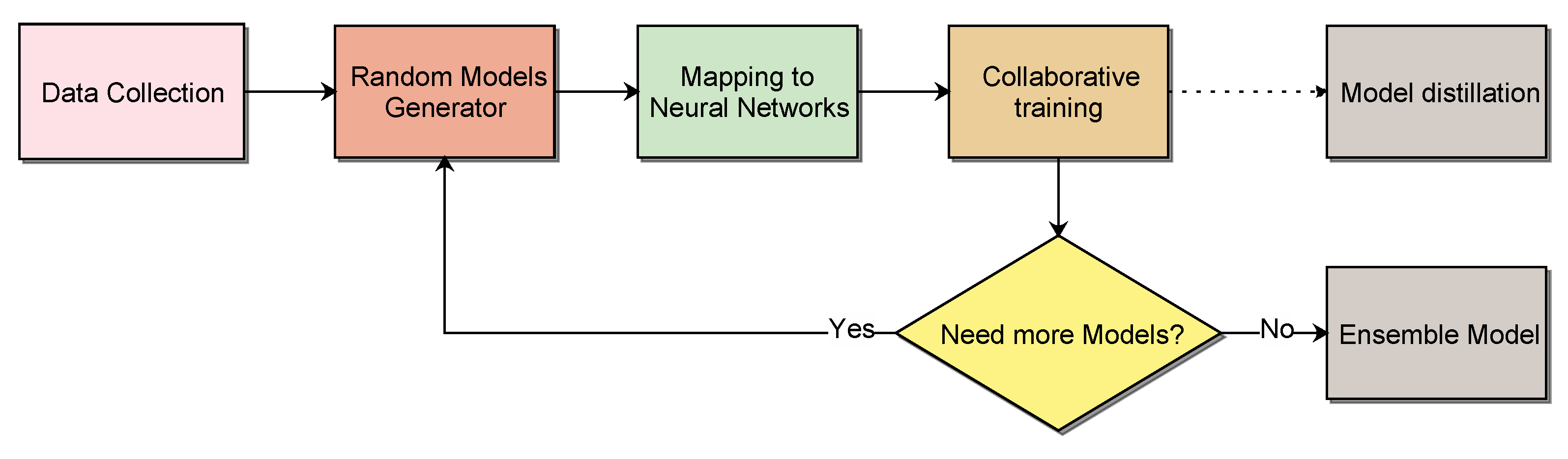
The collaborative training is achieved by transferring knowledge with function-preserving from the model labeled as a teacher after training for a few iterations to the next model labeled as a student, which continues until the end of the chain. The whole process is repeated until the training of each model is converged. This training strategy significantly improved the performance of each model in the chain compared to training each model individually. Figure 1 shows the components of the proposed system.
The main contributions of this paper can be summarized as follows. First, the paper provides a novel way to create an ensemble model generated from a random graph algorithm. The proposed method is different from all existing ensemble methods, which are either based on traditional approaches, such as bagging, or implicitly creating an ensemble, such as dropout. Second, the paper provides a novel way to train the generated ensemble model by introducing collaboration between models. This shows significant improvement of the training models compared to the independent training of models. Third, the paper provides a novel model distillation approach in which the smallest model has a similar performance to the largest model in the generated model chain with a much smaller number of parameters. Fourth, the experiments are accomplished on three datasets (CIFAR-10, CIFAR-100, and TinyImageNet) to validate and show the significance of the proposed method.
2. Related Work
Ensemble learning is traditionally used to improve the overall generalization of the machine learning model by combining a set of diverse models to make the final decision. The diversity among the models could be injected by using different sub-sampling of the training data or stacking different models together. However, these general ensemble strategies are not taking deep learning capabilities into account.
Creating an ensemble of deep learning models can be categorized into implicit and explicit ensemble approaches. In explicit ensemble approaches, a set of deep models is explicitly created and trained separately. In order to improve the training process, in [16], the authors introduced the MotherNets model where a mother model was created from an ensemble by capturing the structural similarity and trained from scratch. Then, the learned model was transferred to the ensemble using function-preserving transformations. The models in the ensemble were then trained using bagging. However, the accuracy of each model was degraded compared to the MotherNets at the beginning of training and needs several iterations to recover.
Our method is close to this one. However, we introduce collaborative learning to train all models simultaneously. This strategy shows a significant improvement in the performance of each model. In [12], the authors proposed a deep mutual learning (DML) method to train an ensemble of models by adding a loss function to match the class posterior probability of all models in the ensemble. In this paper, we propose transfer learning with functional-preserving as a way of communication between models.
In implicit ensemble approaches, an ensemble is generated by training a single model with multiple training options. Dropout [17] is implicitly creating an ensemble of different sub-networks of a single model by dropping out a set of hidden nodes randomly on each iteration during training. DropConnect [18] works similarly, but it drops out weights instead of nodes during training. Then, the stochastic depth method [19] is proposed, which shortens the network during training by randomly dropping layers instead of nodes or weights and replacing them with identity functions. This implicitly creates an ensemble of networks with different depths during the testing time.
Recently, Snapshot ensemble [20] was introduced to generate an explicit ensemble from a single training process by tacking snapshots at various local minima produced by using a cyclic annealing schedule. The implicit ensemble is usually seen as a regularization method to reduce overfitting. Moreover, it can be used along with an explicit ensemble approach.
Knowledge distillation refers to training a smaller model (i.e., a student) to mimic the performance of a large model or an ensemble (i.e., a teacher). The student model is trained with an additional loss function to prompt the model to be identical to the teacher model. Various distillation methods have been introduced to examine different types of loss functions [21,22], different forms of teacher model [23,24], and the best way to train the student model [25,26]. For example, in [27], the authors introduced an approach (called AvgMKD) to distill knowledge from multiple teachers.
They integrated softened outputs of each teacher equally and imposed constraints on the intermediate layers of the student models using the relative dissimilarity learned from the teacher networks. However, by treating each teacher equally, the differences between teacher models could be lost. In [14], authors proposed an adaptive multi-teacher knowledge distillation method (named AMTML-KD) that extended the previous method by adding an adaptive weight for each teacher model and transferring the intermediate-level knowledge from hidden layers of the teacher models to the student models.
Another distillation variant is co-distillation [12,13] where the teacher and student had the same network architecture and were trained in parallel using distillation loss before any model converged. It has shown improvement in the speed of model training and its accuracy. Zhang’s method [12] can be seen as co-distillation of models that have different architectures. Our proposed method can be seen as the co-distillation of randomly generated models, but the distillation method is using transfer learning instead of an extra loss function.
Knowledge transfer is another student–teacher paradigm, where the knowledge is transferred by passing the parameters of each layer of a trained teacher model to the student model as initialization before beginning training the student model. The knowledge is transferred from a smaller model to a larger model with function preserving transformations to accelerate the training of the student model. The expansion of the student network can be achieved by increasing its depth, width, or kernel size. Net2Net [10] expands the depth of the teacher model by adding new layers with identity functions, while Network Morphism [11] derives the new kernels after expanding the model that preserves the function of the teacher model.
In this paper, we used knowledge transfer to train the the models generated by a random graph algorithm. We construct a chain of random-based models and train collaboratively with function-preserving transformations where each model is working as a teacher model to the next model in the chain. The knowledge transfer allows us to train each model in the chain based on the knowledge of each other and, therefore, go beyond the local minima.
3. Proposed Method
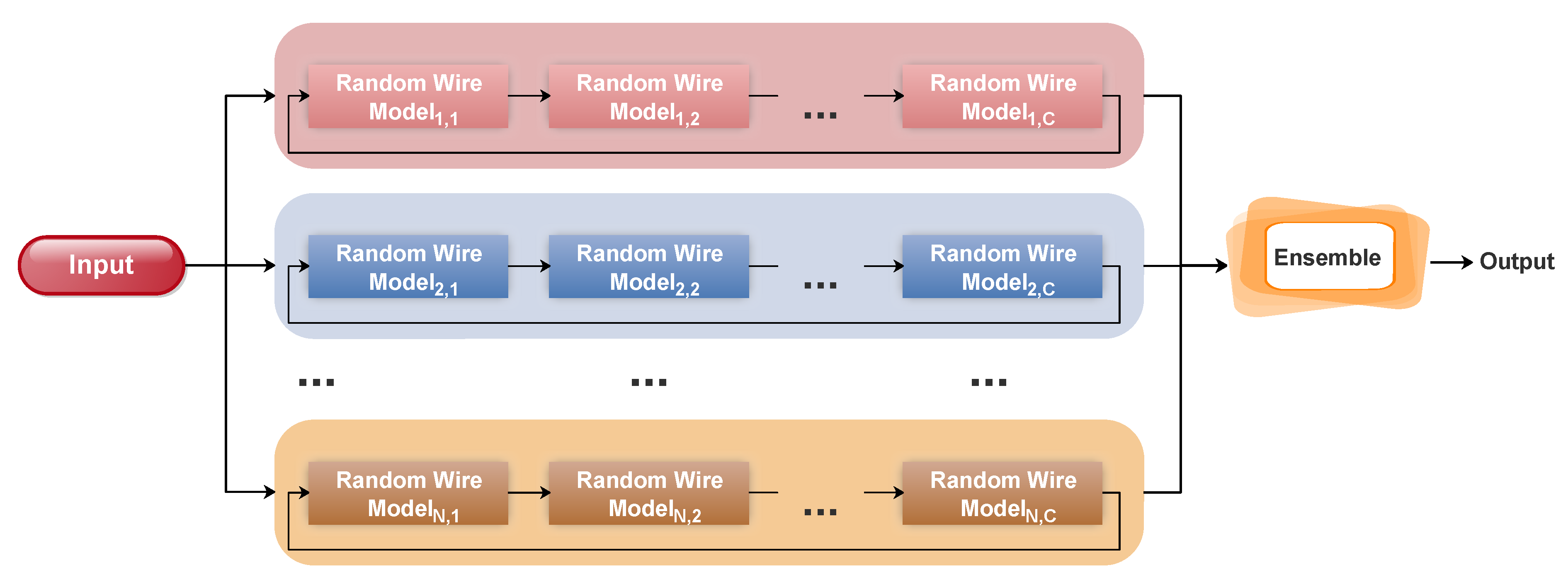
Figure 2 shows an overall view of the proposed system. We creat a set of chains of randomly wired neural network models. In each chain, a large random model is defined based on a random graph algorithm and then iteratively pruned to create a set of small random models. These models are mapped to neural networks and trained collaboratively using functional-preserving transfer learning. Finally, the models in all chains are combined to form a robust model.
3.1. Randomly Wired Neural Networks
Finding the optimal neural network architecture is challenging and usually requires careful hand designing of neural network blocks. Defining how network wiring is achieved is one of the reasons for the recent advances of deep learning models. Early deep learning models have series-like wiring where a set of convolutional blocks are connected sequentially.
Each convolutional block has one or more convolutional layers with non-linear activation functions and is followed by a pooling layer for spatial downsampling. By exploring more in connectivity patterns, models, such as ResNet and DenseNet, have achieved superior performances in many computer vision tasks. Another way to investigate the wiring patterns is by using NAS to search for both the wiring and operation in each block. However, the wiring patterns in all these models are manually designed, and the searching space is limited to a small subset of all possible connections. In this paper, we adopted a randomly wired method [6] to generate network architecture.
In randomly wired neural networks, the wiring patterns between neural network blocks are generating based on a random graph algorithm. First, the method generates a random graph based on one of these algorithms: Erdos-Renyi (ER) [28], Barabasi-Albert (BA) [29], or Watts-Strogatz (WS) [30]. This graph is composed of a number of nodes and edges between them without any restriction about how the graph is generated. Then, the generated graph is mapped to functional neural networks and finally trained on the input data. In this paper, we used the WS model to generate a random graph. The WS model generated a graph that had small-world network properties.
This works by creating a ring network of N nodes where each node is connected to its nearest K neighbors that are equally distributed on both sides of the node, followed by probabilistic rewiring the rightmost edges of every node in the graph to the target node. Rewiring is achieved by uniformly selecting a random target node without creating any self-loop or duplicated edge. The generated random graph is converted to a directed graph by simply making the edge direction from the node that has the lower-index to the higher-indexed node where each node has an index that is assigned sequentially in clockwise order.
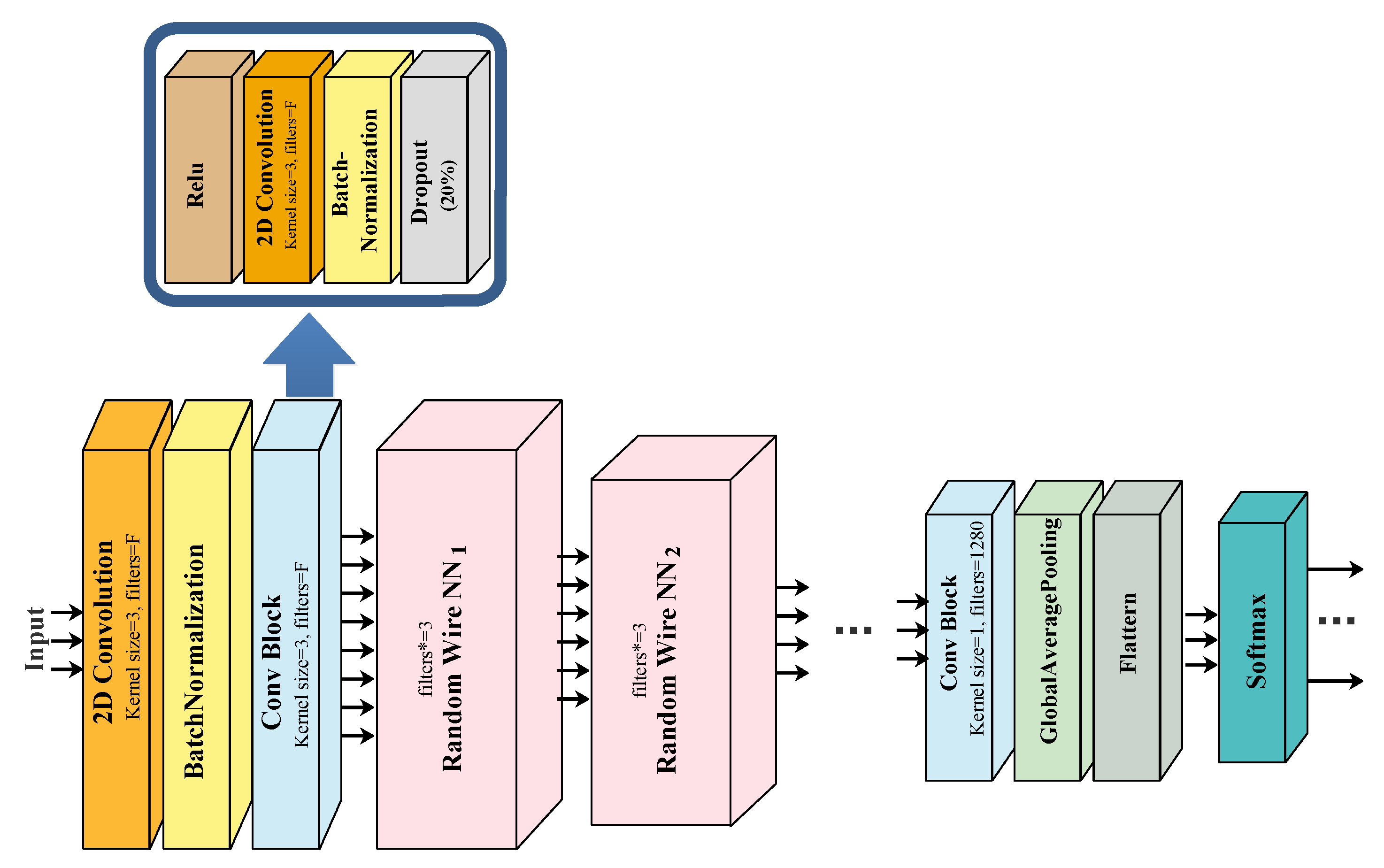
In the mapped neural networks, the edges of the generated random graph define the direction of data flow in the neural network. Each node corresponds to a convolutional block that consists of four layers: ReLU activation, 2D-convolution, batch normalization, and dropout. The convolutional operation is performed by a kernel. The output feature map at node ℓ is defined by convolving kernel with the aggregated input feature map as follows:
where is the bias term. The feature maps generated by the convolution operation go through batch normalization for better regularization. Batch normalization is normalizing the feature maps with the mean and standard deviation of the mini-batch. The dropout layer is helpful in reducing the over-fitting problem by randomly removing a specified proportion of nodes during training the network. Any node has one or more input and also one or more output edges. The input of each node is aggregated as a weighted sum of all the input feature maps where weights are positive and learnable parameters and then go through ReLU activation as follows:
ReLU returns zero if it receives a negative value or the input value itself otherwise.
The output edges are carried by the same copy of the computations accomplished by the node. The random graph could have some input nodes and some output nodes. To maintain the data flow, each input node receive the same data that comes from the previous layer or stage. For the output nodes, an average of all the output nodes is computed and transferred to the next stage in the full neural network model.
The deep learning model usually consists of many stages that gradually decrease the size of the feature map. Here, each stage is represented by a random graph that is stacked together to form the model. Figure 3 shows the architecture of a randomly wired neural network. It starts with one convolutional layer, batch normalization, and convolutional block. Then, for each stage, a random graph is generated and mapped to the neural network space. The final layers are a convolutional block, global average pooling, and a softmax layer. The softmax layer is defined by applying the exponential function to each element of the input vector z and normalizing the result:
where K is the number of classes. The number of filters is gradually increased, starting from 78 for the first two convolutional layers, and then the number is increased by a factor for each stage. The number of filters is set to 1280 at the final convolutional layer before the global average pooling.
3.2. Deep Collaborative Learning
DCL refers to a set of deep learning models that are collaboratively learning from each other. DCL includes three concepts creating function-preserving models, swapping teacher–student training, and forming an ensemble model. First, a chain of deep random models is created based on the idea of function preserving transformations across models. This chain of deep random models is generated from one large random deep model by iteratively removing nodes from the previous model in the chain. The chain-like construction allows transferring knowledge previously acquired by a smaller model to a larger one to improve the performance of each other.
The models in the chain are trained together using teacher–student learning to reduce the degradation of the knowledge transfer. Each model is working as a teacher to the next model in the chain, where the smallest model is at the beginning of the chain and the largest model is at the end. A set of chains of models can be combined to build an ensemble model that improves the final performance on different image classification tasks. The ensemble of chains differs from traditional ensemble methods.
First, it requires a lower number of models to achieve decent results. The diversity between models is achieved by a simple change in the model architecture compared to using data sub-sampling techniques or having more complex architecture, and finally our ensemble model can converge faster than the traditional ensemble methods.
3.2.1. Function-Preserving Models
The idea of function-preserving transformations has been introduced in Net2Net and Network morphism [10,11] where a teacher model (i.e., small model) was fully trained on the training set and then transferred its knowledge to a student model (i.e., large model) that preserved the same functionally of the teacher model. The student model could be larger than the teacher model in the number of feature maps (i.e., wider), the number of layers (i.e., deeper), or increasing the kernel size. However, these methods were applied to hand-designed deep learning models that were trained separability without collaboration. In this paper, we propose function-preserving transformation in chain-like random deep models that are collaborative learning.
We started by generating a large random graph model with N nodes and iteratively pruning nodes from the random graph until reaching the base graph to create a chain of models. The pruned node was selected randomly from any graph node except the output nodes. Since the graph may have many input nodes, the input nodes can be pruned. The edges of the pruned node that connect to its input and outputs nodes were also removed. In order to maintain the graph structure, new edges were defined to connect the input and output nodes of the pruned one directly if there was no existing connection.
These new edges were added to both the pruned graph and all the previous graphs to assure that the pruned (i.e., smaller) graph was a part of the all larger graphs to facilitate the function-persevering transfer learning. The pruned node is now considered as a newly added node in the original graph. This new node was added as an input to some existing nodes according to the edges between them. Equation (2) can be redefined as:
where is the feature map of the new node, and is the weight. The is initially set to zero; however, it is learnable during the training process.
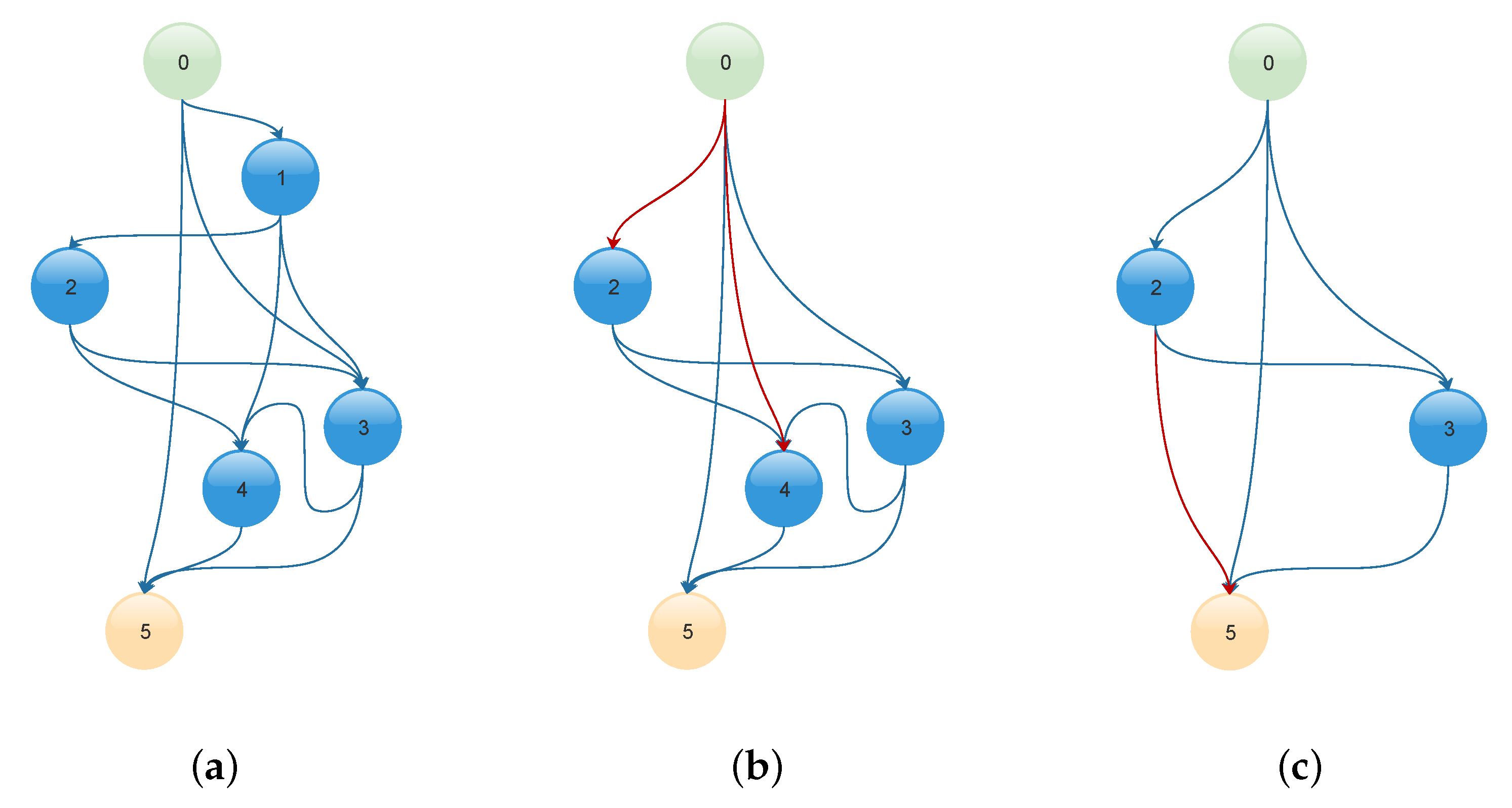
The created new graph is now the same as the original graph but without the pruned nodes and its connections. The pruned graph has a number of nodes equal to . The process was repeated until reaching the base graph, which is the graph with the smallest number of nodes. The chain generator algorithm is given in Algorithm 1. After creating the chain of random graphs, this was mapped to deep learning models as described in Section 3.1. Figure 4 shows a demo of a chain of random models. Here, a random graph of six nodes was created and iteratively pruned one node each time (two times).
| Algorithm 1: Generate a chain of random models |
 |
3.2.2. Collaborative Learning
In our method, the chain of models is trained jointly and in a collaborative way. Starting from the base model, each model in the chain is working as a teacher to the next model until reaching the largest model at the end of the chain. The learning is accomplished in a close loop where the last model passes its knowledge to the first model, and this process is repeated until the training convergence. The collaborative learning strategy is to transfer the knowledge of the model gained after a few epochs of training to the next model. Since the teacher model is already included in the student model, this transfer learning with function-preserving is possible.
The neural network blocks in both models are mapped based on matching nodes between the two random graphs that the models are built accordingly. Initially, all the edge weights are set to zero and convolutional kernels are randomly defined. After a few epochs, all the learned edge weights and kernels are copied to the next model to be trained for a few epochs and so on. This is repeated until training convergence, where each model has resumed its training from the last epoch reached.
The collaborative training algorithm is presented in Algorithm 2. The list of random graphs E needs to be inverted; therefore, we begin training with the smallest model. The function MappingNN(E) takes the random graphs and converts them to the neural network models as discussed in Section 3.1. Each model is trained for a few epochs and then transfers its weights to the next model. Ep is set to five epochs, and the total number of epochs T is 60.
| Algorithm 2: Deep Collaborative Learning |
 |
3.2.3. Ensemble Model
Training the chain of collaborative deep random models leads to a better and faster converge for each model. However, it tends to make the models produce similar results because of the function-preserving transformations that share all the knowledge learned by one model to the other models. The ensemble model requires a set of diverse models to produce an effective result. Here, we created a set of small chains of models and combine them together. Each minimum chain contained three models that were trained collaboratively using the DCL method.
This strategy significantly improved the ensemble performance of the chains of random models. Each model had a softmax layer to produce the probability output of each class. The last step was combining the output of all models in the chain to produce the final decision. Many combination techniques can be used, such as sum rule, product rule, majority voting, and stacking. Here, we compare sum rule, product rule, and majority voting, as these methods have no parameters and do not require any further training. The product rule is multiplying the output probabilities of each model.
where M is the total number of models in the ensemble. The sum rule has a more relaxed behavior by taking the sum instead of the multiplication.
The majority voting is similar to the sum rule, but it adds a vote to each class based on the model prediction.
where is a binary vector that contains 1 to the chosen class by the model and zero otherwise. It is hard voting as no final probability is computed for each class.
4. Results and Discussion
4.1. Datasets & Implementation Details
The proposed method is evaluated on 3 datasets for image classification: CIFAR-10, CIFAR-100, and TinyImageNet. CIFAR-10 and CIFAR-100 datasets consist of 50K training images and 10K testing images associated with 10 and 100 class labels, respectively. Each image is in RGB format and has a dimension of pixels. TinyImageNet classification [31] is similar to the classification challenge of the ImageNet [32] with 200 classes for training. Each class has 500 training images. TinyImageNet includes 100K training images and 10K testing images. The images are colored with dimensions of pixels.
For all datasets, we used the same experimental settings as follows. We set the mini-batch size to 100, the total number of epochs to 60, and the initial learning rate to 0.1. The learning rate dropped by 0.1 every 20 epochs. The data augmentation is utilized by including horizontal flips, randomly shift images horizontally and vertically, and randomly rotate images. We run the experiments five times and report the best result.
4.2. Results on CIFAR-10, CIFAR-100, and TinyImageNet
We conducted several experiments to compare between training the generated chain of models with and without deep collaborative learning. We evaluated the proposed method as a knowledge distillation model and compared it with the state-of-the-art-methods. We also compared our collaborative learning method with the MotherNets method [16], and finally, the proposed method was assessed as an ensemble model.
In the first experiment, a chain of three models was defined by iteratively pruning one node from each stage of the initial generated random graphs as described in Algorithm 1. Each model had two stages with 16 initial nodes, and the number of filters was increased by a factor of 3. The first and the second row in Table 1 report the results when the chain of models trained independently and with the DCL. The first model (i.e., number 1) in the chain refers to the smallest model and the last model (i.e., number 3) refers to the largest model in terms of the number of nodes.
The proposed collaborative learning significantly improved the performance of each model in the chain compared to the individual training of each model. DCL improved the average accuracy of each model by 1.35%, 1.31%, and 3.16% on CIFAR-10, CIFAR-100, and TinyImageNet, respectively. For example, the third model in the chain had an accuracy of , , and on CIFAR-10, CIFAR-100, and TinyImageNet, respectively, compared to , , and for the independent training.
Next, we compared between the DCL and the MotherNets [16] as shown in Table 1 rows 2 and 3. In MotherNets, the first model was fully trained and considered as the mother model so that it transfered its learning to the rest of the models. The DCL had a significant improvement over MotherNets. For example, the accuracy of the second model in that chain was , , and on CIFAR-10, CIFAR-100, and TinyImageNet, respectively, compared to , , and using MotherNets. The MotherNets models had a limited improvement compared with the independent training.
To show the advantage of the proposed method as a model distillation, we trained a chain of six models based on two random graphs (i.e., one per stage) of 16 nodes on CIFAR-10 and CIFAR-100 as shown in Table 2. The smallest model (i.e., model no. 1) had fewer parameters and approximated floating-point operations (FLOPS) compared with the largest model (i.e., model no. 6).
The DCL demonstrated significant improvement in the accuracy of each model. For CIFAR-10, The accuracy of models 1, 2, and 6 using the DCL was , , and compared to , , and for the independent training models. The accuracy difference between the first and the last model in the DCL trained chain was only with less in the number of parameters of the first model compared to the last model. While the accuracy difference between the second and the last model was , and the second model had less in the number of parameters.
DCL showed a significant advantage as a model distillation by transferring the knowledge between models with different sizes of parameters. For CIFAR-100, The DCL models 1, 2, and 6 had an accuracy of , , and compared to , , and using the independent training of each model. The accuracy difference between the first and the last model and between the second and the last model was and , respectively.
The proposed method was compared to three knowledge distillation methods; DML [12], AvgMKD [27], and AMTML-KD [14] as shown in Table 3. Each method was used to train three student models on the CIFAR-10, CIFAR-100, and TinyImageNet datasets. DML trained three student networked collaboratively to learn with each other and without using any teacher models. AvgMKD and AMTML-KD used three teacher models based on ResNet, VGG-19, and DenseNet. Table 3 reports the accuracy difference before and after using the knowledge distillation method.
The performance of the proposed method outperformed other state-of-the-art methods. On CIFAR-10, the proposed DCL method increased the accuracy of student model 1, 2 and 3 by , , and , respectively, compared to , , and for DML, , , and for AvgMKD, and , , and for AMTML-KD. On CIFAR-100, The DCL method achieved an average improvement of compared to , , and for DML, AvgMKD, and AMTML-KD, respectively. The AMTML-KD was slightly better than the DCL for the first student model only. On TinyImageNet, The DCL method significantly improved the performance of all student models. The average accuracy difference of DCL was compared to , , and for DML, AvgMKD, and AMTML-KD, respectively.
The ensemble model was tested using different combination techniques: sum rule (SR), product rule (PR), and majority voting (MV), as shown in Table 4. Two chains of random models were trained independently and using DCL. These chains were based on a random graph of eight nodes and contained two stages. The increasing factor of filters was set to 2 for the first chain and 3 for the second one. The PR and SR showed better performance compared to MV.
For example, the results of the ensemble using PR of DCL models were , , and on CIFAR-10, CIFAR-100, and TinyImageNet, respectively, compared to , , and for using SR and , , and for using MV. Here, we used PR to report the results of the ensemble model. The accuracy of the ensemble of models trained independently (, , and on CIFAR-10, CIFAR-100, and TinyImageNet, respectively) was much higher than each model in the chain (the best results were , , and ).
These results indicate that a small change in the model architecture improved the diversity between the models and, therefore, the ensemble accuracy. The ensemble of DCL models demonstrated better performance compared with the ensemble of independent models. The results of the DCL ensemble on CIFAR-10, CIFAR-100, and TinyImageNet were , , and compared to , , and for the ensemble of independent training models. Table 4 also shows the accuracy of each individual model with and without DCL. The collaborative learning of a small set of models significantly enhanced the accuracy of each model over the independent training.
In the next experiment, we examined a different number of models to form an ensemble on CIFAR-10, CIFAR-100, and TinyImageNet, and we report the ensemble accuracy of the independent training and DCL in Table 5. The ensemble of DCL models was significantly higher than the independent training of models on the CIFAR-10, and TinyImageNet datasets. The models in the ensemble were created by changing the number of nodes, the number of filters, and/or the number of stages.
We started with a simple configuration of the ensemble by setting the number of stages to 2, the number of nodes to 8, and the increasing factor of filters to 2. Then, we gradually changed these parameters to increase the number of models in the ensemble. The increasing factor of filters was altered between 2 and 3. The number of nodes was increased to 16 and 32, and later the number of stages was set to 3. Note, each configuration resulted in three models that were trained collaboratively using DCL.
On CIFAR-10, the best result of DCL was reached with an ensemble of 18 models () compared to the independent training (). On CIFAR-100, the accuracy of an ensemble of 15, 18, and 21 DCL models was , , and , respectively. For the independent training, the ensemble accuracy was , , and , respectively.
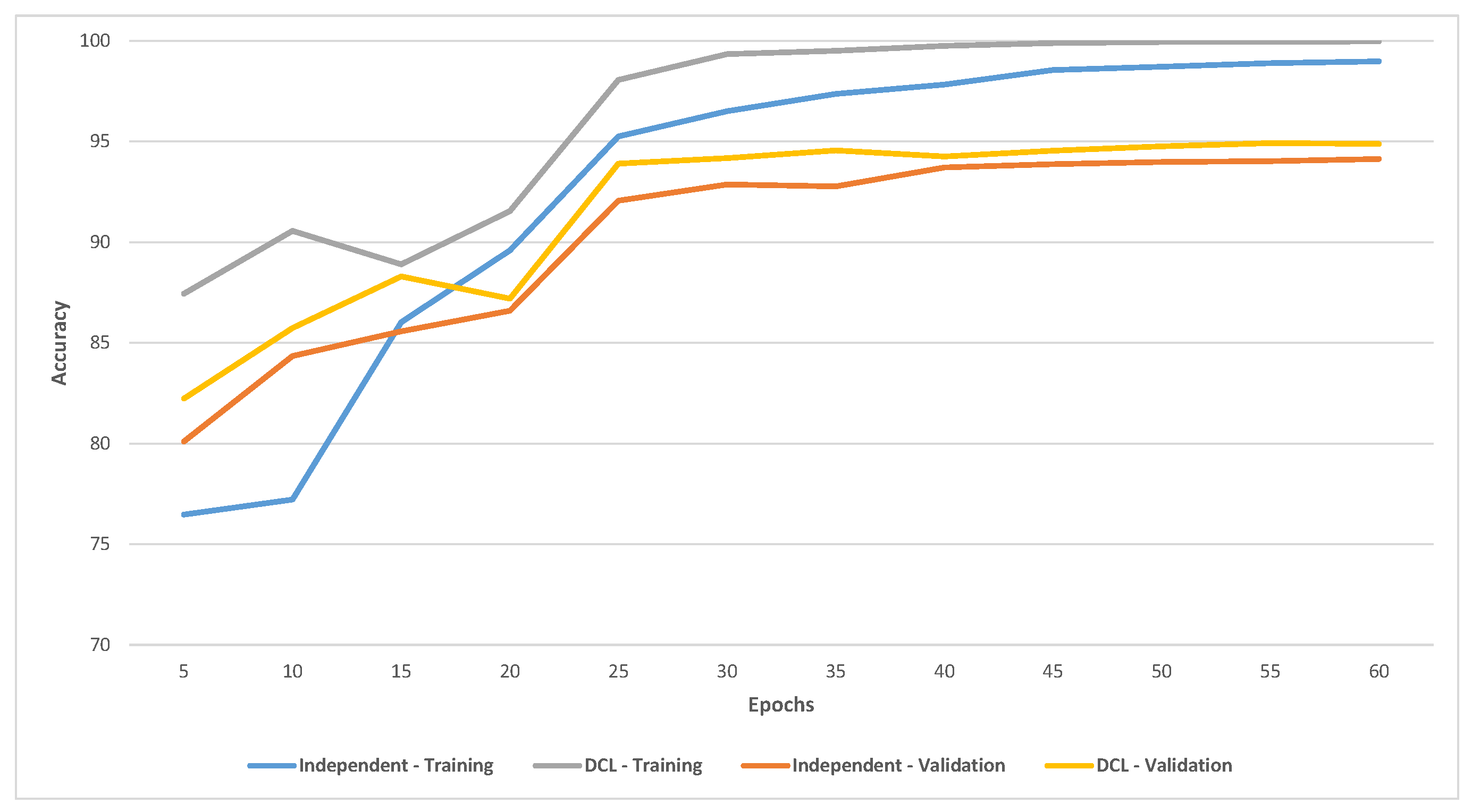
On TinyImageNet, the DCL significantly improved the accuracy of the ensemble. The accuracy of an ensemble of 9, 15, and 21 DCL models was , , and compared to , , and for the independent training, respectively. Figure 5 shows the training and validation accuracy on CIFAR-10 of the ensemble of six independent training and DCL models (using 32 nodes). DCL had significantly better accuracy for training and validation and converged faster than independent training.
5. Conclusions
We presented a deep collaborative method for training a chain of randomly wired neural networks to improve the performance of each model. The proposed method can be used to produce a strong ensemble model and to achieve a robust knowledge distillation. We created a large randomly wired deep learning model based on a random graph and iteratively pruning nodes to create a chain of function-preserving models. The chain of models was trained collaboratively by using transfer learning.
The proposed training method resulted in the smallest model in the chain having a similar performance to the largest model. The proposed method was evaluated on the CIFAR-10, CIFAR-100, and TinyImageNet datasets. The experimental results showed the effectiveness of the proposed method as a model distillation and an ensemble model. In the future, we will extend our method to other recognition tasks and explore more training techniques and design patterns that may lead to more powerful networks.
Author Contributions
Conceptualization, E.E. and X.X.; methodology, E.E.; software, E.E.; validation, E.E.; formal analysis, X.X.; investigation, E.E.; resources, X.X.; data curation, X.X.; writing—original draft preparation, E.E. and X.X.; writing—review and editing, E.E. and X.X.; visualization, E.E. and X.X.; supervision, X.X.; project administration, X.X.; funding acquisition, E.E. and X.X. Both authors have read and agreed to the published version of the manuscript.
Funding
This research is funded by the Cymru COFUND Fellowship.
Data Availability Statement
The CIFAR-10 and CIFAR-100 datasets used in this paper are openly available and can be found here https://www.cs.toronto.edu/~kriz/cifar.html. The TinyImageNet dataset can also be downloaded from http://cs231n.stanford.edu/tiny-imagenet-200.zip.
Conflicts of Interest
The authors declare no conflict of interest.
References
- Szegedy, C.; Liu, W.; Jia, Y.; Sermanet, P.; Reed, S.; Anguelov, D.; Erhan, D.; Vanhoucke, V.; Rabinovich, A. Going Deeper with Convolutions; CVPR: Boston, MA, USA, 2015; pp. 1–9. [Google Scholar]
- Simonyan, K.; Zisserman, A. Very Deep Convolutional Networks for Large-Scale Image Recognition; ICLR: San Diego, CA, USA, 2015. [Google Scholar]
- He, K.; Zhang, X.; Ren, S.; Sun, J. Deep Residual Learning for Image Recognition; CVPR: Las Vegas, NV, USA, 2016; pp. 770–778. [Google Scholar]
- Huang, G.; Liu, Z.; Van Der Maaten, L.; Weinberger, K.Q. Densely Connected Convolutional Networks; CVPR: Honolulu, HI, USA, 2017; pp. 4700–4708. [Google Scholar]
- Wistuba, M.; Rawat, A.; Pedapati, T. A survey on neural architecture search. arXiv 2019, arXiv:1905.01392. [Google Scholar]
- Xie, S.; Kirillov, A.; Girshick, R.; He, K. Exploring Randomly Wired Neural Networks for Image Recognition; ICCV: Seoul, Korea, 2019; pp. 1284–1293. [Google Scholar]
- Lee, S.; Purushwalkam, S.; Cogswell, M.; Crandall, D.; Batra, D. Why M heads are better than one: Training a diverse ensemble of deep networks. arXiv 2015, arXiv:1511.06314. [Google Scholar]
- Szegedy, C.; Vanhoucke, V.; Ioffe, S.; Shlens, J.; Wojna, Z. Rethinking the Inception Architecture for Computer Vision; CVPR: Las Vegas, NV, USA, 2016; pp. 2818–2826. [Google Scholar] [CrossRef] [Green Version]
- Hinton, G.; Vinyals, O.; Dean, J. Distilling the knowledge in a neural network. arXiv 2015, arXiv:1503.02531. [Google Scholar]
- Chen, T.; Goodfellow, I.; Shlens, J. Net2net: Accelerating learning via knowledge transfer. arXiv 2015, arXiv:1511.05641. [Google Scholar]
- Wei, T.; Wang, C.; Rui, Y.; Chen, C.W. Network Morphism; ICML: New York City, NY, USA, 2016; pp. 564–572. [Google Scholar]
- Zhang, Y.; Xiang, T.; Hospedales, T.M.; Lu, H. Deep Mutual Learning; CVPR: Salt Lake City, UT, USA, 2018; pp. 4320–4328. [Google Scholar]
- Song, G.; Chai, W. Collaborative Learning for Deep Neural Networks; NIPS: Montreal, QC, Canada, 2018; pp. 1832–1841. [Google Scholar]
- Liu, Y.; Zhang, W.; Wang, J. Adaptive multi-teacher multi-level knowledge distillation. Neurocomputing 2020, 415, 106–113. [Google Scholar] [CrossRef]
- Guo, Q.; Wang, X.; Wu, Y.; Yu, Z.; Liang, D.; Hu, X.; Luo, P. Online Knowledge Distillation via Collaborative Learning; CVPR: Seattle, WA, USA, 2020. [Google Scholar]
- Wasay, A.; Hentschel, B.; Liao, Y.; Chen, S.; Idreos, S. Mothernets: Rapid Deep Ensemble Learning. In Proceedings of the Conference on Machine Learning and Systems (MLSys), Austin, TX, USA, 2–4 March 2020. [Google Scholar]
- Srivastava, N.; Hinton, G.; Krizhevsky, A.; Sutskever, I.; Salakhutdinov, R. Dropout: A simple way to prevent neural networks from overfitting. J. Mach. Learn. Res. 2014, 15, 1929–1958. [Google Scholar]
- Wan, L.; Zeiler, M.; Zhang, S.; Le Cun, Y.; Fergus, R. Regularization of Neural Networks Using Dropconnect; ICML: Atlanta, GA, USA, 2013; pp. 1058–1066. [Google Scholar]
- Huang, G.; Sun, Y.; Liu, Z.; Sedra, D.; Weinberger, K.Q. Deep Networks with Stochastic Depth; ECCV: Amsterdam, The Netherlands, 2016; pp. 646–661. [Google Scholar]
- Huang, G.; Li, Y.; Pleiss, G.; Liu, Z.; Hopcroft, J.E.; Weinberger, K.Q. Snapshot ensembles: Train 1, get m for free. arXiv 2017, arXiv:1704.00109. [Google Scholar]
- Romero, A.; Ballas, N.; Kahou, S.E.; Chassang, A.; Gatta, C.; Bengio, Y. Fitnets: Hints for thin deep nets. arXiv 2014, arXiv:1412.6550. [Google Scholar]
- Tian, Y.; Krishnan, D.; Isola, P. Contrastive representation distillation. arXiv 2019, arXiv:1910.10699. [Google Scholar]
- Balan, A.K.; Rathod, V.; Murphy, K.P.; Welling, M. Bayesian Dark Knowledge; NIPS: Montreal, QC, Canada, 2015; pp. 3438–3446. [Google Scholar]
- Yuan, L.; Tay, F.E.; Li, G.; Wang, T.; Feng, J. Revisit Knowledge Distillation: A Teacher-free Framework. arXiv 2019, arXiv:1909.11723. [Google Scholar]
- Sau, B.B.; Balasubramanian, V.N. Deep model compression: Distilling knowledge from noisy teachers. arXiv 2016, arXiv:1610.09650. [Google Scholar]
- Mirzadeh, S.I.; Farajtabar, M.; Li, A.; Ghasemzadeh, H. Improved knowledge distillation via teacher assistant: Bridging the gap between student and teacher. arXiv 2019, arXiv:1902.03393. [Google Scholar]
- You, S.; Xu, C.; Xu, C.; Tao, D. Learning from Multiple Teacher Networks. In Proceedings of the 23rd ACM SIGKDD International Conference on Knowledge Discovery and Data Mining, Halifax, NS, Canada, 13–17 August 2017; pp. 1285–1294. [Google Scholar] [CrossRef]
- Erdös, P.; Rényi, A. On the evolution of random graphs. Publ. Math. Inst. Hungary Acad. Sci. 1960, 5, 17–61. [Google Scholar]
- Albert, R.; Barabási, A.L. Statistical mechanics of complex networks. Rev. Mod. Phys. 2002, 74, 47. [Google Scholar] [CrossRef] [Green Version]
- Watts, D.J.; Strogatz, S.H. Collective dynamics of ‘small-world’ networks. Nature 1998, 393, 440–442. [Google Scholar] [CrossRef] [PubMed]
- Le, Y.; Yang, X. Tiny ImageNet Visual Recognition Challenge; Technical Report; Stanford University: Stanford, CA, USA, 2015. [Google Scholar]
- Russakovsky, O.; Deng, J.; Su, H.; Krause, J.; Satheesh, S.; Ma, S.; Huang, Z.; Karpathy, A.; Khosla, A.; Bernstein, M.; et al. ImageNet Large Scale Visual Recognition Challenge. Int. J. Comput. Vis. 2015, 115, 211–252. [Google Scholar] [CrossRef] [Green Version]
Figure 1.
The components of the proposed system. First, we collect the training labeled data. Second, a chain of randomly wired models is created. Third, the models are mapped to neural networks and, then, trained collaboratively. Finally, we produce a set of models that are co-distillation. We could also produce a multiple set of random models and combine them to form a robust ensemble model.

Figure 2.
The proposed system overview. First, multiple sets of a chain of randomly wired models are created. These models are mapped to neural networks and trained collaboratively using functional-preserving transfer learning. Finally, the models in all chains are combined to form a robust ensemble model.

Figure 3.
The architecture of a randomly wired neural network.

Figure 4.
An example of a chain of random models. (a) The first generated random graph has six nodes and one input (number 0) and one output (number 5). (b) The random graph after removing node number 1. (c) The random graph after removing node number 4. The compensating edges (shown in red color) will be added later to all previous graphs.

Figure 5.
Training and validation accuracy of the ensemble of six independent training and DCL models on CIFAR-10.
Figure 5.
Training and validation accuracy of the ensemble of six independent training and DCL models on CIFAR-10.


Table 1.
A comparison between independent training, MotherNets, and DCL between models on CIFAR-10, CIFAR-100, and TinyImageNet.
Table 1.
A comparison between independent training, MotherNets, and DCL between models on CIFAR-10, CIFAR-100, and TinyImageNet.
| CIFAR-10 | CIFAR-100 | TinyImageNet | |||||||
|---|---|---|---|---|---|---|---|---|---|
| 1 | 2 | 3 | 1 | 2 | 3 | 1 | 2 | 3 | |
| Independent | 93.84 | 94.13 | 93.88 | 76.12 | 75.44 | 75.55 | 57.59 | 57.18 | 57.49 |
| DCL | 95.28 | 95.24 | 95.38 | 76.98 | 77.05 | 77.02 | 60.54 | 60.42 | 60.79 |
| MotherNets [16] | 93.85 | 93.58 | 94.08 | 76.73 | 76.17 | 74.95 | 57.40 | 56.51 | 57.63 |
Table 2.
Evaluation of DCL and independent training on CIFAR-10 and CIFAR-100 using a chain of six random models.
Table 2.
Evaluation of DCL and independent training on CIFAR-10 and CIFAR-100 using a chain of six random models.
| CIFAR-10 | CIFAR-100 | |||||
|---|---|---|---|---|---|---|
| Models | Parameters | FLOPS | Independent | DCL | Independent | DCL |
| 1 | 93.73 | 94.81 | 74.78 | 76.96 | ||
| 2 | 94.00 | 94.99 | 74.52 | 77.10 | ||
| 3 | 93.81 | 94.99 | 75.14 | 77.64 | ||
| 4 | 93.73 | 94.89 | 75.50 | 77.53 | ||
| 5 | 94.19 | 95.12 | 75.48 | 77.38 | ||
| 6 | 93.80 | 95.10 | 75.44 | 77.45 | ||
Table 3.
A comparison between state-of-the-art distillation methods and DCL on CIFAR-10, CIFAR-100, and TinyImageNet. The values denote the accuracy difference between the baseline model and the distillation model.
Table 3.
A comparison between state-of-the-art distillation methods and DCL on CIFAR-10, CIFAR-100, and TinyImageNet. The values denote the accuracy difference between the baseline model and the distillation model.
| CIFAR-10 | CIFAR-100 | TinyImageNet | |||||||
|---|---|---|---|---|---|---|---|---|---|
| 1 | 2 | 3 | 1 | 2 | 3 | 1 | 2 | 3 | |
| DCL | 1.44 | 1.11 | 1.5 | 0.86 | 1.61 | 1.47 | 2.95 | 3.24 | 3.30 |
| DML [12] | 0.41 | 0.23 | 0.05 | 0.30 | 0.37 | 0.44 | 0.68 | 0.33 | 0.40 |
| AvgMKD [27] | 0.72 | 0.61 | 0.35 | 0.95 | 0.71 | 0.69 | 0.93 | 0.68 | 0.65 |
| AMTML-KD [14] | 1.35 | 1.18 | 0.99 | 1.70 | 1.56 | 1.34 | 1.57 | 1.40 | 1.30 |
Table 4.
A comparison of an ensemble of DCL models and independent models on CIFAR-10, CIFAR-100, and TinyImageNet.
Table 4.
A comparison of an ensemble of DCL models and independent models on CIFAR-10, CIFAR-100, and TinyImageNet.
| Chain of Models 1 | Chain of Models 2 | |||||||||
|---|---|---|---|---|---|---|---|---|---|---|
| 1 | 2 | 3 | 1 | 2 | 3 | MV | SR | PR | ||
| CIFAR-10 | Independent | 92.40 | 92.89 | 93.37 | 93.64 | 93.08 | 93.87 | 94.19 | 94.24 | 94.16 |
| DCL | 93.54 | 94.11 | 93.92 | 94.13 | 94.64 | 94.46 | 94.51 | 94.69 | 94.76 | |
| CIFAR-100 | Independent | 71.31 | 72.50 | 72.65 | 74.53 | 74.11 | 74.48 | 76.19 | 76.55 | 76.66 |
| DCL | 72.54 | 73.22 | 73.26 | 75.21 | 75.74 | 75.44 | 75.48 | 76.42 | 76.70 | |
| TinyImageNet | Independent | 53.04 | 54.14 | 55.47 | 56.98 | 57.73 | 58.77 | 59.88 | 60.65 | 60.56 |
| DCL | 56.6 | 57.65 | 57.63 | 60.36 | 60.85 | 60.36 | 60.47 | 62.19 | 62.48 | |
Table 5.
Evaluation of different sizes of DCL model ensembles on CIFAR-10, CIFAR-100, and TinyImageNet.
Table 5.
Evaluation of different sizes of DCL model ensembles on CIFAR-10, CIFAR-100, and TinyImageNet.
| Number of Models | |||||||
|---|---|---|---|---|---|---|---|
| 6 | 9 | 12 | 15 | 18 | 21 | ||
| CIFAR-10 | Independent | 94.16 | 94.63 | 94.75 | 94.83 | 94.82 | 94.77 |
| DCL | 94.76 | 95.18 | 95.47 | 95.60 | 95.84 | 95.77 | |
| CIFAR-100 | Independent | 76.66 | 77.46 | 77.90 | 78.12 | 78.28 | 78.19 |
| DCL | 76.70 | 77.67 | 78.81 | 79.31 | 79.57 | 79.71 | |
| TinyImageNet | Independent | 60.56 | 61.18 | 61.70 | 61.90 | 61.64 | 62.02 |
| DCL | 62.48 | 63.55 | 64.77 | 65.08 | 65.04 | 66.39 | |
Publisher’s Note: MDPI stays neutral with regard to jurisdictional claims in published maps and institutional affiliations. |
© 2021 by the authors. Licensee MDPI, Basel, Switzerland. This article is an open access article distributed under the terms and conditions of the Creative Commons Attribution (CC BY) license (https://creativecommons.org/licenses/by/4.0/).
Share and Cite
MDPI and ACS Style
Essa, E.; Xie, X. Deep Collaborative Learning for Randomly Wired Neural Networks. Electronics 2021, 10, 1669. https://doi.org/10.3390/electronics10141669
AMA Style
Essa E, Xie X. Deep Collaborative Learning for Randomly Wired Neural Networks. Electronics. 2021; 10(14):1669. https://doi.org/10.3390/electronics10141669
Chicago/Turabian StyleEssa, Ehab, and Xianghua Xie. 2021. "Deep Collaborative Learning for Randomly Wired Neural Networks" Electronics 10, no. 14: 1669. https://doi.org/10.3390/electronics10141669
Note that from the first issue of 2016, this journal uses article numbers instead of page numbers. See further details here.