
A Comparison Study of Observed and the CMIP5 Modelled Precipitation over Iraq 1941–2005

1
Department of Civil and Environmental Engineering, Colorado State University, Fort Collins, CO 80523, USA
2
Department of Civil Engineering, Faculty of Science and Engineering, Swansea University Bay Campus, Swansea SA1 8EN, UK
3
Department of Civil Engineering, College of Engineering, Kufa University, Kufa 54003, Iraq
*
Author to whom correspondence should be addressed.
Atmosphere 2022, 13(11), 1869; https://doi.org/10.3390/atmos13111869
Submission received: 22 September 2022
/
Revised: 4 November 2022
/
Accepted: 6 November 2022
/
Published: 9 November 2022
(This article belongs to the Special Issue Hydroclimate in a Changing World: Recent Trends, Current Progress and Future Directions)
Abstract
:This paper presents an analysis of the annual precipitation observed by a network of 30 rain gauges in Iraq over a 65-year period (1941–2005). The simulated precipitation from 18 climate models in the CMIP5 project is investigated over the same area and time window. The Mann–Kendall test is used to assess the strength and the significance of the trends (if any) in both the simulations and the observations. Several exploratory techniques are used to identify the similarity (or disagreement) in the probability distributions that are fitted to both datasets. While the results show that large biases exist in the projected rainfall data compared with the observation, a clear agreement is also observed between the observed and modelled annual precipitation time series with respect to the direction of the trends of annual precipitation over the period.
1. Introduction
Studying precipitation trends is an essential step in assessing the impact of climate change on hydrological processes. A substantial change in the amount of precipitation can lead to severe conditions of flooding and droughts. It is also important to examine such trends for water resource planning since water demand may be affected; thus, strategies and operations for the water supply need to be adjusted accordingly.
While the trend of recorded observations of hydro-meteorological variables, such as precipitation, has been widely studied using long-term observation datasets, e.g., [1], scenario-based climate projections are still a preferred source for most studies on the future trends of climate change. More recently, the Fifth Climate Model Inter-comparison Project CMIP5 [2] published a rich set of climate simulations produced by several key metrological centres in the world, which offers an updated and improved (in both accuracy and resolution) collection of outputs of climate models for many downstream impact studies, e.g., [3,4,5,6].
The post-industrial period, particularly the 20th century, has been the focus of many studies on the trend of hydro-climatic variables. Generally, these studies aimed to establish a link between the so-called anthropogenic greenhouse effect and the change in climate, as indicated by the key variables. Moreover, the baseline period was chosen by many studies as observation records became abundant. The studied areas range from global to regional scales. To name just a few: New et al. [7] showed that, in the 20th century, precipitation has significantly changed in various parts of the world, and Griggs and Noguer [8] and Xu et al. [9] pointed out that the average annual rainfall considerably increased by 7–12% in the high and middle latitudes in the northern hemisphere during the 20th century.
Several statistical techniques have also been employed to detect the trend and the shift of climatological variables, as reported in Martinez et al. [10]. There are two main families of methods for determining trends, parametric and non-parametric, with non-parametric methods being preferred over parametric ones, as the former is less likely to be affected by the outliers and does not assume a predefined distribution for datasets or homogeneity [11]. The statistical test of Mann–Kendall, i.e., the MK test [12,13], has often been utilized to evaluate the trends of rainfall [14,15].
Most studies have been carried out on the trend of observed hydro-meteorological variables; few are focused on the trend analysis of simulated variables such as precipitation projection from climate models. Rather, many studies make use of “snapshots” from climate projections to indicate the difference (hence change) between the projected value of the variable in question and its current values, without revealing the process or temporal trend associated with such change.
On the other hand, researchers tend to use projected, scenario-defined variables from climate model simulations, notably, precipitation, to drive other models for impact studies. Errors or biases in these simulated variables have been widely recognized in this type of application. While sophisticated bias correction methods have also been developed to cope with this situation, little attention has been paid to the trend of those simulated variables either with or without bias correction. It is very plausible that an overall quantity-fit projection after bias correction may not be able to reproduce the trend revealed by the observations; to some extent, this would be more of a concern in projection-driven climate impact studies.
Trend analysis of precipitation data on the regional and global scales has been studied by many researchers all over the world. Readers can refer to Palomino-Lemus et al. [16], Sharmila et al. [17] and Palizdan et al. [18]. Global climate models are broadly utilized to create current and project future climate conditions [19,20]. This is essential to investigate and evaluate the models’ performance in simulating precipitation to develop adaptation strategies to reduce uncertainties in projecting precipitation in the future [21].
The Coupled Model Intercomparison Project Phase 5 (CMIP5) comprises more comprehensive global climate models than its predecessors, enabling researchers to address many research questions [22]. The assessment methods for different models’ performance have progressed from traditional qualitative methods to quantitative methods [23]. Some research has assessed models based on some traditional statistical methods, such as spatial correlation coefficients [24], linear trend analysis [20] and standard deviation [25].
Several climate studies that primarily used GCMs to estimate the future of the earth’s climate system indicated changes in the climate from the regional scale [26,27] to global scale [28,29]. Deng et al. [30] evaluated nine CMIP5 datasets under different RCP future scenarios for the projections of summer and spring precipitation for the period of 2013–2050 over the Yangtze River basin in China. The precipitation projections revealed significant positive linear trends of spring precipitation under the RCP2.6 and RCP8.5 scenarios, while summer precipitation is shown to be undergoing an inter-annual change. Mehran et al. [31] used volumetric hit index (VHI) analysis with 34 CMIP5 GCMs to reproduce observed precipitation across the globe. The GCMs showed good agreement with the observed monthly time series. However, reproducing the observed precipitation over some subcontinental and arid regions was problematic. Their finding proves the allegation that GCMs have weaknesses when it comes to the representation of observed precipitation on small spatial scales and short temporal scales, e.g., [27].
Nikiema et al. [32] compared and evaluated the multi-model ensembles of CMIP5 and CORDEX and found that while CORDEX failed to outperform the temperature simulated by the CMIP5 ensembles, it considerably enhanced the simulation of historical summer precipitation and provided a more realistic fine-scale features tied to land use and local topography. Long-range correlation (LRC) is an effective way to evaluate CMIP5 models’ performance in global precipitation and has been employed in many aspects of climate systems, such as precipitation [33] and air temperature [34].
The above studies have contributed immensely to the assessment of the performance of GCMs and RCMs in reproducing the observed climatology of various regions, but very few focus on places with limited observed climate data, such as Iraq. Therefore, assessing the performances of several GCMs from CMIP5 over Iraq will contribute significantly to the efforts in climate modelling over the region.
The study presented in this paper takes a different approach from those used by many previous studies in trend analysis. It first investigates the observed precipitation in Iraq over a 65-year period (1941–2005); this is then compared with the modelled precipitation from an array of 18 climate models from the latest CMIP5 projects. Both the spatial and temporal distribution trends are studied alongside a bias correction procedure applied to the modelled data. Further, several exploratory statistical techniques are used to check the similarity between the observed and modelled precipitation.
2. Materials and Methods
2.1. Study Area
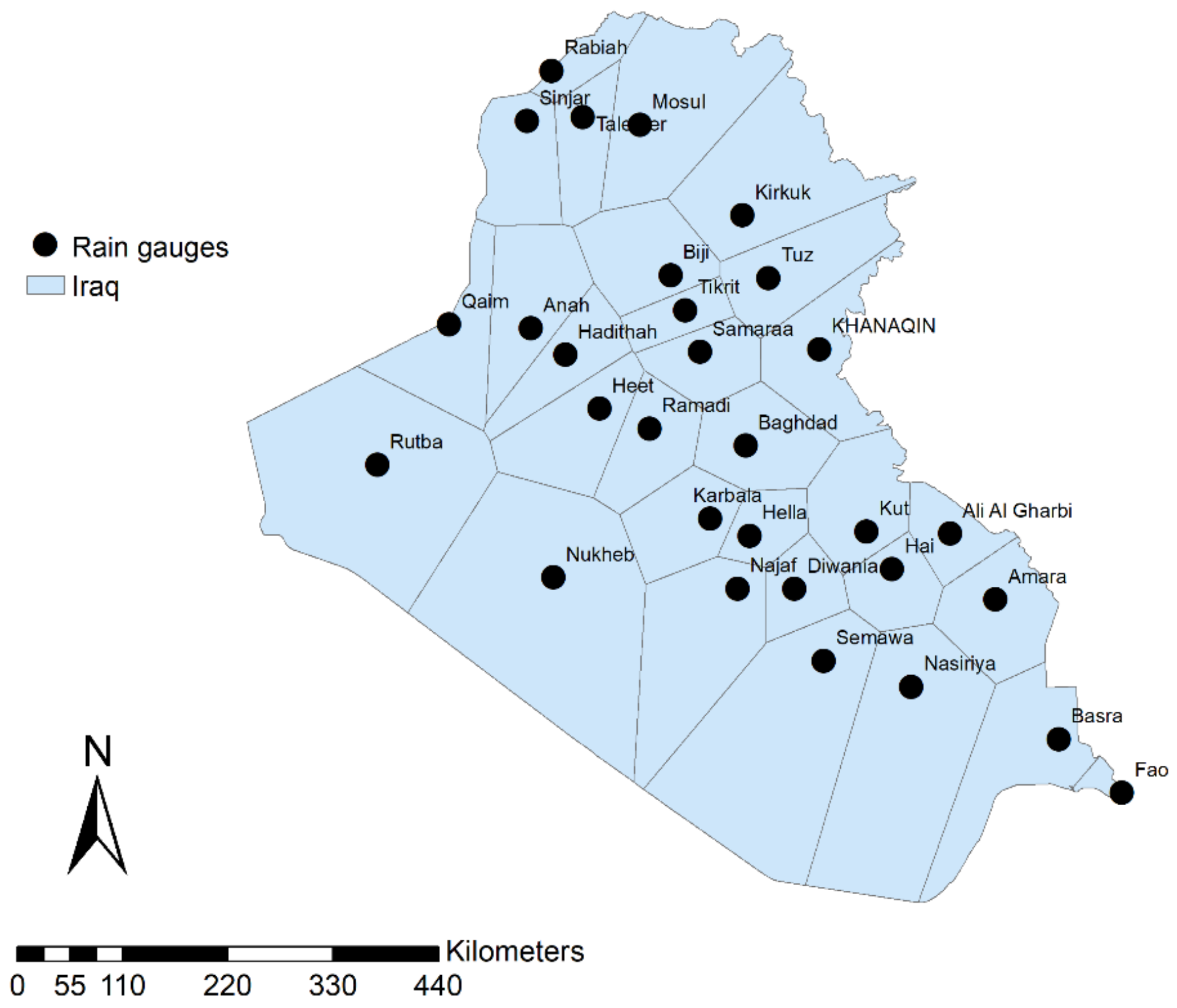
Located within the southwest of the continent of Asia, Iraq shares land borders with Turkey in the north, Kuwait and Saudi Arabia in the south, Iran in the east and Syria and Jordan in the west (Figure 1). Iraq comprises a total area of 437,065 km2. The climate is mainly described as a semi-arid, subtropical, and continental type; meanwhile, the north and northeast parts have a Mediterranean climate [35]. Iraq has a rainy season in cold months, from December to February, excluding the north area of the country, where the seasonal precipitation takes place from November to April.
The yearly precipitation in Iraq is estimated to be 216 mm countrywide on average; regionally, it has a range of less than 100 mm over the southern region to 1200 mm in the northeast of the country [35]. Summer in Iraq is hot and dry to extremely hot with a shade temperature of over 43 °C that falls at night to 26 °C. Winter is cold, with a day temperature of about 16 °C, dropping at night to 2 °C [36]. According to the FAO [35], Iraq can be divided into four agroecological zones:
- (1)
- Semi-arid and arid zones with a Mediterranean climate (zone 1 in Figure 1): The annual precipitation varies between 700 and 1000 mm and occurs between October and April. The country has cold and rainy winters, while summers are hot and dry; they are even torrid up to quite high altitudes. This zone mainly covers the north of the country. This is the only region in Iraq that receives a considerable amount of precipitation.
- (2)
- Steppes with winter rainfall of 200–400 mm annually (zone 2 in Figure 1): Summers are extremely hot, and winters are cold. In the cold season of the year, some depressions can pass that carry moderate precipitation.
- (3)
- The desert zone/northwest of Mesopotamia (zone 3 in Figure 1) has a high temperature in summer and less than 200 mm of yearly rainfall.
- (4)
- The irrigated area which covers the region between the Euphrates and Tigris rivers (zone 4 in Figure 1). This region has a desert or semi-desert climate, with mild winters and extremely hot summers.
The land elevation decreases from the northeast mountainous parts near the Iranian and Turkish borders (3450 m) to the desert regions in the south and west near the Syrian and Saudi Arabian borders (a few meters above sea level).
2.2. Precipitation Data
Due to the limited and restricted availability of data, only monthly precipitation data from 30 rain gauges over the period of 1941–2005 are obtained from the General Organization of Meteorology and Seismic Monitoring in Iraq, and these are illustrated in Figure 1 alongside a summary presented in Table 1. The gaps due to missing data are filled using the inverse distance weighted interpolation method (IDW). The annual average precipitation over the study area is then interpolated over the country, ranging from 92 to 376 mm, as shown in Figure 2.
The statistical summary of the annual precipitation is illustrated in Figure 3 for zones 2, 3 and 4. The annual precipitation over zone 2 ranges from 35 to 700 mm with an average of circa 300 mm for the period of 1941–2005, whereas for zone 3 and 4, the range is 3–347 mm/year with an average of around 127 mm/year.
Areal precipitation is obtained using the Thiessen polygon method based on the 30 rain gauges, illustrated in Figure 4. Additionally, the box plot of the average precipitation in Iraq for 7 decadal periods is examined as follows: 1941–1950, 1951–1960, 1961–1970, 1971–1980, 1981–1990, 1991–2000 and 2001–2005. The box plot in Figure 5 is used to investigate the annual and seasonal patterns: winter (combination of December, January and February (DJF)), spring (sum of March, April and May (MAM)) and autumn (sum of September, October and November (SON)) of average precipitation obtained from 30 stations, as defined previously. Apparently, the pattern of precipitation differs at several temporal bands and between seasons, as shown in Figure 5.
The Coupled Model Inter-Comparison Phase Five (CMIP5) experiments consist of several numerical climate simulation models with various constraints, such as land use changes, environmental pollution, and volcanic emissions. CMIP5 [2] is divided into two major components:
- (1)
- Long-term experiments (century and longer); and
- (2)
- Near-term experiments (decadal prediction).
There are 28 meteorological centres around the world that supply CMIP5 climate model outputs with different settings of near- and extended-future scenarios and different groups of spatial and temporal resolutions. In this paper, 18 models from the CMIP5 project that can produce long-term scenarios are used. There are four main future scenarios when considering the climate data: RCPs 2.6, RCPs 4.5, RCPs 6.0, and RCPs 8.5 [2]. Detailed information on the CMIP5 models used in this study is described in Table 2.
2.3. The Goodness-of-Fit Tests (GOFs)
In this paper, three statistical GOF tests are used to evaluate the selected CMIP5 model simulations for comparison with the observed precipitation based on monthly time series for the period of 1941–2005. The criteria used for the evaluation include:
- Mean error (ME), which can be calculated as follows:where is the observed rainfall at time t and is the simulated rainfall at time t.
- Mean absolute error (MAE):
- Root mean square error (RMSE), which can be calculated as:
- Correlation coefficient (r): This index measures the linear relationship between two time series with a range between −1 and 1, where −1 indicates a perfect negative correction, 0 no correlation at all and 1 a perfect positive correlation. It can be calculated as follows:
2.4. Fitting of Probability Distributions
It is imperative to know the underlining distributions of both observations and simulated data. This serves two purposes:
- (1)
- To check if the two datasets are statistically consistent; and
- (2)
- To identify any changes in the probability distribution of simulated data for the future.
The skewness–kurtosis graph, also known as the Cullen and Frey graph technique, is applied to select the most suitable distribution type to fit the dataset before the data are fitted with the chosen distribution types. Information on this method is provided in [37]. It gives the choice of the best fit for an unknown distribution according to the kurtosis and skewness levels. It utilizes predefined distributions such as normal and lognormal to achieve a moment fitting. It can also show the maximum likelihood of data and evaluate the goodness of fit (GOF).
In this technique, the x-axis is the square of skewness, and the y-axis is kurtosis. The input data model is represented as a solid circle in this study, as demonstrated in the sections. Several symbols illustrate different types of distribution. If the skewness and kurtosis of the observation circle and the known distribution symbol are similar, it means the observation and the modelled data might have the same or even a similar distribution.
In this study, 8 predefined probability distributions are considered, including beta, uniform, exponential, gamma, normal, logistic, log-normal and Weibull distributions. The R statistical package “fitdistrplus” [38] is employed to conduct the analysis for both the observed rainfall and selected CMIP5 models.
2.5. Bias Correction
A bias correction based on quantile mapping is applied to the CMIP5 models that have the best fit using the goodness-of-fit criteria mentioned in Section 2.3. Studies such as Maraun [39] and Eden et al. [40] found that climate projection simulations from GCMs often come with a substantial number of uncertainties as well as biases and errors. Undoubtedly, the confidence in the direct use of GCM simulations has been adversely affected, such that no reliable conclusions can be drawn using uncorrected GCM simulation data. However, sophisticated bias and error correction of GCMs data have gone beyond the scope of this paper. The simple quantile mapping [41] technique is used to adjust the climate data over the baseline period.
Quantile mapping is a bias correction technique through which the modelled variable is adjusted through equating the cumulative distribution function CDFs of both the observation and simulated dataset. To achieve this, the following transform function is implemented:
where and are cumulative distribution functions of both the observed and the simulated time series, and is the modelled variable at time (t). Typically, the quantile mapping algorithm will be presented through quantile–quantile (Q-Q) plot (e.g., dotty plot between empirical quantile of simulated and observed data if the CDF (simulated data) and inverse CDF (observed data) are empirically projected from the data.
Like other statistical bias correction approaches, the quantile mapping method presumes that climate models’ biases are stationary. Further information about this method can be found in Maraun et al. [41]. The quantile mapping technique divides the cumulative distribution function data into discrete portions, and an individual quantile mapping is implemented as a correction into each segment, resulting in a better-fitted transfer function.
2.6. Mann–Kendall Trend Test (MK)
The non-parametric trend test, Mann–Kendall [12,13], has been extensively used in hydrology and climatology studies to investigate significance slope or trend since it is simple and robust. Let X = (x1, x2, x3…, xn) be the time series dataset; the Mann–Kendall statistics S can be computed as follows:
where
The variance for the Mann- Kendall trend test can be calculated as follows:
where:
- : is the number of data points;
- : is the number of tied groups for the month;
- : is the number of data in the group for the month.
It is revealed that, when following the null hypothesis (no trend) H0, S will follow a normal distribution and thus can be used to test the hypothesis with a confidence level of 1 − α/2. The overall projected trend of slope β, which is the Theil–Sen slope [42,43], is calculated as the measured dataset Y over time X. The individual slope estimator is calculated as follows:
The Mann–Kendall trend test will be carried out using R statistical package rkt [44].
3. Results
3.1. Statistical Comparison between Observed and Modelled Precipitation
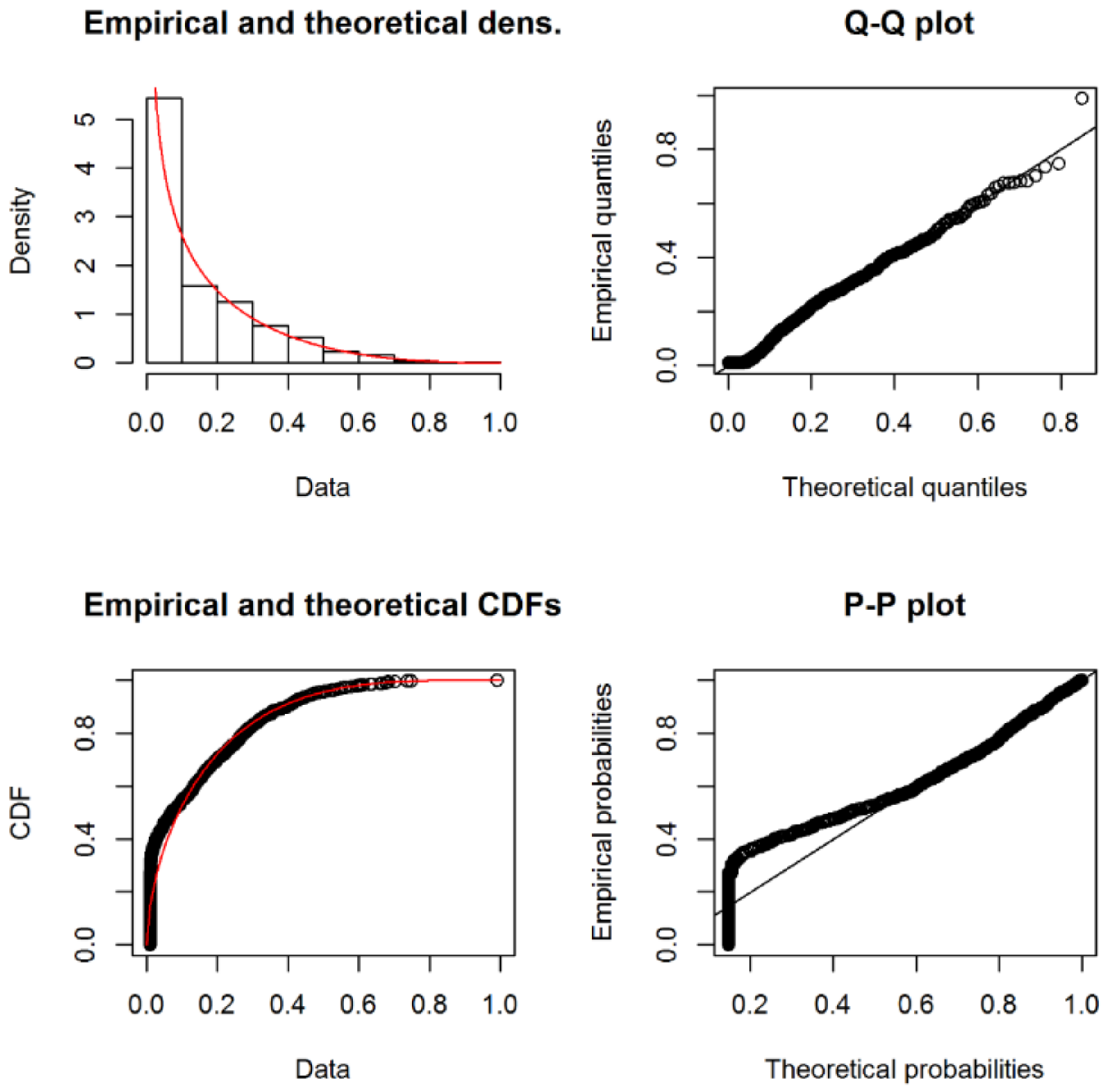
The skewness–kurtosis graph (Cullen and Frey plot) technique is employed to check whether the average areal rainfall of observations and CMIP5 models are drawn from the same family of theoretical distribution. The monthly time series for the observations and the 18 models of CMIP5 are evaluated against eight theoretical distributions. As can be seen in Figure 6, the observed rainfall lies within the region of beta distribution. Further assessment of the observed rainfall against the beta distribution is conducted using the Q-Q plot, p-p plot, empirical and theoretical PDFs and CDFs. The results show that the observation fits well to the beta distribution seen in Figure 7, as indicated by the parameters of both the observed data and the bootstrapped data (i.e., via resampling the observed data), being situated well within the shaded area representing the beta distribution. This is further confirmed by Figure 7, which shows an overall good fit of the beta distribution to the observation dataset.
The 18 model-simulated precipitations are evaluated based on their ME, MAE, RMSE, correlation coefficient (r) and fitting of theoretical distribution for the monthly areal average rainfall of Iraq, as illustrated in Table 3. The comparison reveals that the bcc-csm1-1, bcc-csm1-1-m, CCSM4, MIROC5 and MRI-CGCM3 models have a relatively better representation of rainfall than the other models.
The areal average of the cumulative rainfall of the observed data and simulated outputs of CMIP5 is shown in Figure 8. The comparison reveals that MRI-CGCM3, CCM4 and MIROC5 have better qualitative estimation than the others, as illustrated in Figure 8, and the statistical comparison in Table 3 also supports this.
The quantile mapping bias correction is applied to the monthly rainfall time series of the five selected models, bcc-csm-1-1, bcc-csm-1-1-m, CCM4, MIROC5 and MRI-CGCM3. Model simulations at the locations of the 30 rain gauges are corrected against the observed time series. The corrected model simulations are then used to produce the areal average time series. The density plots of the areal average of the corrected modelled precipitation and the observations reveal a general good agreement between the simulated and observed precipitation in terms of the shapes and the parameters, as shown in Figure 9. However, it is interesting to see that the mode and the skewness of the observed data are not captured well by the modelled data, which may be due to the bias correction applied.
3.2. Trend Analysis of Precipitation
The trend of annual precipitation is evaluated using the Mann–Kendall test for the observed rainfall and the five selected models. The comparison is carried out both in a point-by-point fashion (as demonstrated in Figure 10, Figure 11, Figure 12 and Figure 13) and for the areal average of the study area (Figure 14). The point-by-point trend comparison at 30 locations shows that some models, e.g., bcc-csm-1-1, bcc-csm-1-1-m and CCM4, demonstrate the same trend direction (decreasing trend) at 19 locations, as revealed in Figure 10. Meanwhile, the MIROC5 model reveals the same trend direction (mix of positive and negative trends) at eight locations, and the MRI-CGCM3 model shows the same trend direction at eight locations, as shown in Figure 10.
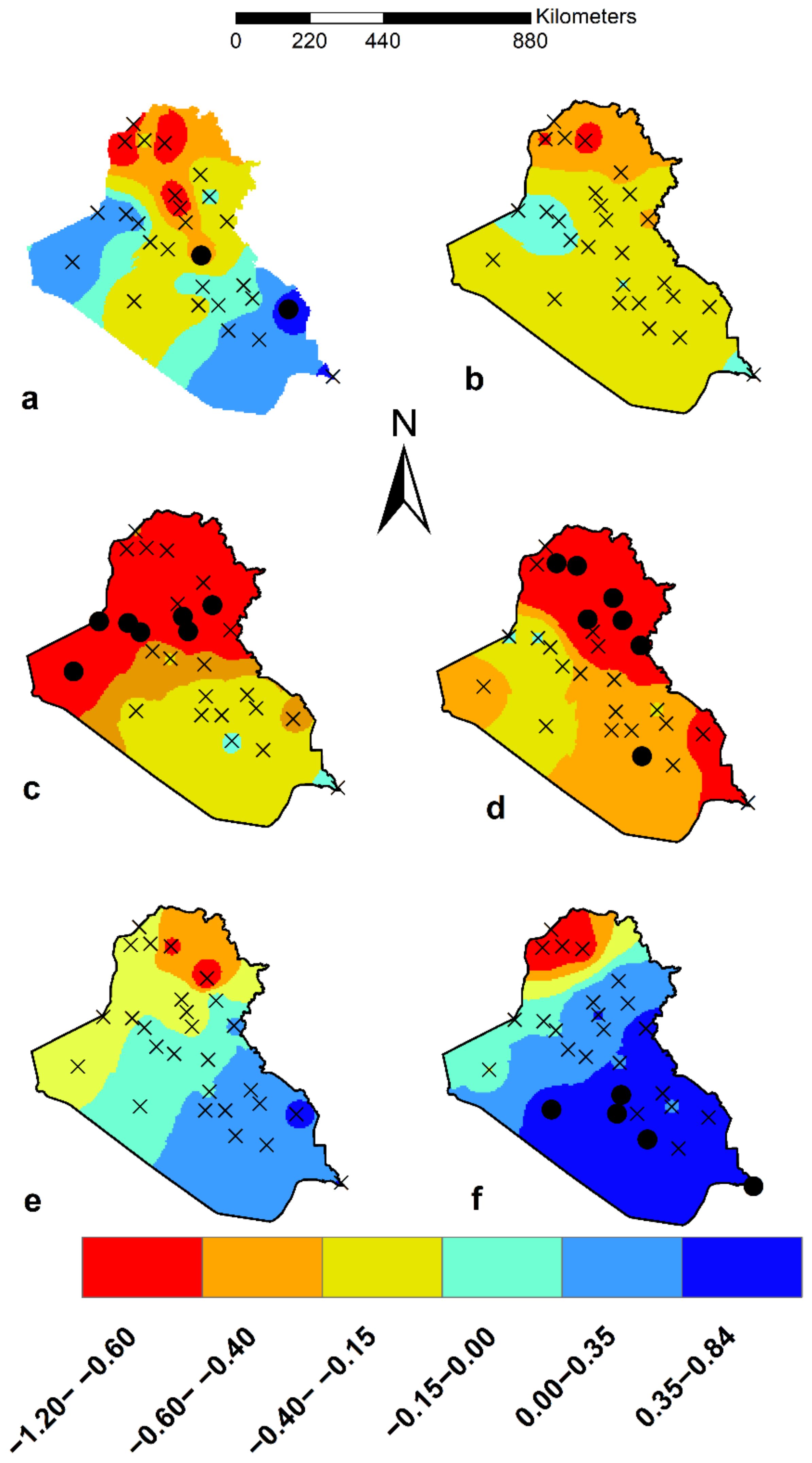
The trends over various zones of the study area are also compared. The spatial distribution of the annual trend is revealed in Figure 11, where the modelled rainfall trends have a different pattern from the observed one. It is also clear from the same figure that there are mixed trends over the study area with a range of (−1.2–0.84) mm/year. Models such as MIROC 5 (Figure 11e) and MRI-CGCM3 (Figure 11f) reveal approximately the same range; however, the spatial distribution is different from that of the observed dataset. The other models (e.g., bcc-csm-1-1, bcc-csm-1-1 m and CCM4 models) exhibit trends of decreasing precipitation over the study area.
Figure 12 shows the comparison of the Mann–Kendal tests of zone 2 for the observed precipitation and the five selected models of CMIP5; it can be concluded that most of the modelled time series are able to demonstrate the same trend direction. In the meantime, for zones 3 and 4, four out of the five selected models produce the same trend direction, as illustrated in Figure 13.
Furthermore, the trend of the average areal precipitation (Figure 14) shows that most models (bcc-csm-1-1, bcc-csm-1-1-m, CCM4 and MIROC5) demonstrate the same trend of decreasing rainfall as that seen for the observed rainfall, except the MRI-CGCM3 model, which shows the opposite trend (positive).
4. Conclusions
In this paper, the focus was set on investigating the annual trend of precipitation over Iraq. The monthly precipitation of 30 rain gauges stations over 65 years, as well as the 18 models from the CMIP5 project with different spatial resolutions, have been collected and used to represent the typical projected climate data in this study. A non-parametric trend test, the Mann–Kendall method, is implemented to test the trends in both datasets, followed by another analysis of the underlying probability distributions. The point-by-point annual rainfall trend comparison reveals that some models (bcc-csm-1-1, bcc-csm-1-1-m and CCM4) are able to capture the trend direction (decreasing trend) at 19 locations. While the MIROC5 model reveals the same trend direction at only eight locations, the MRI-CGCM3 model shows the same trend direction at eight locations. It can be reasonably concluded from the findings that the projected precipitation shows substantial bias and low correlation with the observed data.
However, an agreement is also seen between the observed and modelled annual precipitation time series with respect to the direction of the trends (positive or negative). Furthermore, the preliminary analysis reveals that the observed data can be fitted well with a beta-type probability distribution. For the modelled precipitation, 8 out of 18 models were able to be fitted using the same type of distribution. It may as well be worth waiting until the resolution of climate models progresses even further to the catchment scale to reduce this scale gap so as to make the climate change impact study more reliable. Nevertheless, the findings of this study cast doubt over the practice of directly using projected precipitation for the study of climate change impact on hydrological processes.
Author Contributions
Conceptualization, S.A.A., Y.X., A.H.A.-R. and H.F.A., methodology Y.X. and S.A.A., formal analysis S.A.A. and Y.X., writing—original draft preparation S.A.A., writing—review and editing, Y.X. Collecting and request of observed precipitation data, A.H.A.-R. and H.F.A. All authors have read and agreed to the published version of the manuscript.
Funding
This research received no external funding.
Acknowledgments
Co-author S.A.A. was supported by the Ph.D. scholarship provided by the Higher Committee for Education Development in Iraq, for which we are grateful. We also thank General Organization of Meteorology and Seismic Monitoring in Iraq and the British Atmospheric Data Centre for the provision of the required datasets to support this study. We would like to thank the anonymous reviewers and the editors for their valuable comments and advice, which have helped to improve the quality of this paper.
Conflicts of Interest
The authors declare no conflict of interest. This work is an extended paper based on a chapter in a Ph.D. thesis.
References
- Zhao, P.; Jones, P.; Cao, L.; Yan, Z.; Zha, S.; Zhu, Y.; Yu, Y.; Tang, G. Trend of Surface Air Temperature in Eastern China and Associated Large-Scale Climate Variability over the Last 100 Years. J. Clim. 2014, 27, 4693–4703. [Google Scholar] [CrossRef]
- Meinshausen, M.; Smith, S.J.; Calvin, K.; Daniel, J.S.; Kainuma, M.L.T.; Lamarque, J.F.; Matsumoto, K.; Montzka, S.A.; Raper, S.C.; Riahi, K.; et al. The RCP Greenhouse Gas Concentrations and Their Extensions from 1765 to 2300. Clim. Change 2011, 109, 213–241. [Google Scholar] [CrossRef] [Green Version]
- Chattopadhyay, S.; Jha, M.K. Hydrological Response Due to Projected Climate Variability in Haw River Watershed, North Carolina, USA. Hydrol. Sci. J. 2016, 61, 495–506. [Google Scholar] [CrossRef]
- Jin, X.; Sridhar, V. Impacts of Climate Change on Hydrology and Water Resources in the Boise and Spokane River Basins1. J. Am. Water Resour. Assoc. 2011, 48, 197–220. [Google Scholar] [CrossRef]
- Chattopadhyay, S.; Edwards, D.R. Long-term trend analysis of precipitation and air temperature for Kentucky, United States. Climate 2016, 4, 10. [Google Scholar] [CrossRef]
- Abdo, K.S.; Fiseha, B.M.; Rientjes, T.H.M.; Gieske, A.S.M.; Haile, A.T. Assessment of Climate Change Impacts on the Hydrology of Gilgel Abay Catchment in Lake Tana Basin, Ethiopia. Hydrol. Process. 2009, 23, 3661–3669. [Google Scholar] [CrossRef]
- New, M.; Todd, M.; Hulme, M.; Jones, P. Precipitation Measurements and Trends in the Twentieth Century. Int. J. Climatol. 2002, 21, 1889–1922. [Google Scholar] [CrossRef]
- Griggs, D.J.; Noguer, M. Climate Change 2001: The Scientific Basis. Contribution of Working Group I to the Third Assessment Report of the Intergovernmental Panel on Climate Change. Weather 2006, 57, 267–269. [Google Scholar] [CrossRef]
- Xu, Z.; Takeuchi, K.; Ishidaira, H.; Li, J. Long-Term Trend Analysis for Precipitation in Asian Pacific FRIEND River Basins. Hydrol. Process. 2005, 19, 3517–3532. [Google Scholar] [CrossRef]
- Martinez, C.; Maleski, J.; Miller, M. Trends in Precipitation and Temperature in Florida, USA. J. Hydrol. 2012, 452, 259–281. [Google Scholar] [CrossRef]
- Sonali, P.; Nagesh Kumar, D. Review of Trend Detection Methods and Their Application to Detect Temperature Changes in India. J. Hydrol. 2013, 476, 212–227. [Google Scholar] [CrossRef]
- Mann, H. Nonparametric Tests against Trend. Econometrica 1945, 13, 245–259. [Google Scholar] [CrossRef]
- Kendall, M.G. Rank Correlation Measures; Charles Griffin: London, UK, 1975. [Google Scholar]
- Tabari, H.; Somee, B.; Zadeh, M. Testing for Long-Term Trends in Climatic Variables in Iran. Atmos. Res. 2011, 100, 132–140. [Google Scholar] [CrossRef]
- Modarres, R.; Sarhadi, A. Rainfall Trends Analysis of Iran in the Last Half of the Twentieth Century. J. Geophys. Res. Atmos. 2009, 114, 1–9. [Google Scholar] [CrossRef]
- Palomino-Lemus, R.; Córdoba-Machado, S.; Gamiz-Fortis, S.R.; Castro-Díez, Y.; Esteban-Parra, M.J. Summer precipitation projections over northwestern South America from CMIP5 models. Glob. Planet. Change 2015, 131, 11–23. [Google Scholar] [CrossRef]
- Sharmila, S.; Joseph, S.; Sahai, A.K.; Abhilash, S.; Chattopadhyay, R. Future projection of Indian summer monsoon variability under climate change scenario: An assessment from CMIP5 climate models. Glob. Planet. Change 2015, 124, 62–78. [Google Scholar] [CrossRef] [Green Version]
- Palizdan, N.; Falamarzi, Y.; Huang, Y.F.; Lee, T.S. Precipitation trend analysis using discrete wavelet transform at the Langat River Basin, Selangor, Malaysia. Stoch. Environ. Res. Risk Assess. 2017, 31, 853–877. [Google Scholar] [CrossRef]
- He, W.P.; Zhao, S.S.; Wu, Q.; Jiang, Y.D.; Wan, S. Simulating evaluation and projection of the climate zones over China by CMIP5 models. Clim. Dyn. 2019, 52, 2597–2612. [Google Scholar] [CrossRef]
- Dong, T.Y.; Dong, W.J.; Guo, Y.; Chou, J.M.; Yang, S.L.; Tian, D.; Yan, D.D. Future temperature changes over the critical Belt and Road region based on CMIP5 models. Adv. Clim. Change Res. 2018, 9, 57–65. [Google Scholar] [CrossRef]
- Lin, L.; Gettelman, A.; Xu, Y.; Wu, C.; Wang, Z.; Rosenbloom, N.; Bates, S.C.; Dong, W. CAM6 simulation of mean and extreme precipitation over Asia: Sensitivity to upgraded physical parameterizations and higher horizontal resolution. Geosci. Model Dev. 2019, 12, 3773–3793. [Google Scholar] [CrossRef]
- Tayler, K.E.; Stouffer, R.J.; Meehl, G.A. An overview of CMIP5 and the experimental design. Bull. Am. Meteorol. Soc. 2012, 93, 485–498. [Google Scholar] [CrossRef] [Green Version]
- Li, Q.; Zhang, L.; Xu, W.; Zhou, T.; Wang, J.; Zhai, P.; Jones, P. Comparisons of time series of annual mean surface air temperature for China since the 1900s: Observations, model simulations, and extended reanalysis. Bull. Am. Meteorol. Soc. 2017, 98, 699–711. [Google Scholar] [CrossRef] [Green Version]
- Tian, D.; Guo, Y.; Dong, W. Future changes and uncertainties in temperature and precipitation over China based on CMIP5 models. Adv. Atmos. Sci. 2015, 32, 487–496. [Google Scholar] [CrossRef]
- Yang, S.; Feng, J.; Dong, W.; Chou, J. Analyses of extreme climate events over China based on CMIP5 historical and future simulations. Adv. Atmos. Sci. 2014, 31, 1209–1220. [Google Scholar] [CrossRef]
- Neumann, R.; Jung, G.; Laux, P.; Kunstmann, H. Climate trends of temperature, precipitation and river discharge in the Volta Basin of West Africa. Int. J. River Basin Manag. 2007, 5, 17–30. [Google Scholar] [CrossRef]
- Kunstmann, H.; Jung, G. Impact of regional climate change on water availability in the Volta basin of West Africa. IAHS Publ. 2005, 295, 75–85. [Google Scholar]
- Parry, M.L.; Canziani, O.; Palutikof, J.; Van der Linden, P.; Hanson, C. (Eds.) Climate Change 2007-Impacts, Adaptation and Vulnerability: Working Group II Contribution to the Fourth Assessment Report of the IPCC (Vol. 4); Cambridge University Press: Cambridge, UK, 2007. [Google Scholar]
- Change, I.C. The physical science basis. In Contribution of Working Group I to the Fifth Assessment Report of the Intergovernmental Panel on Climate Change; IPCC: Geneva, Switzerland, 2013; p. 1535. [Google Scholar]
- Deng, H.; Luo, Y.; Yao, Y.; Liu, C. Spring and summer precipitation changes from 1880 to 2011 and the future projections from CMIP5 models in the Yangtze River Basin, China. Quat. Int. 2013, 304, 95–106. [Google Scholar] [CrossRef]
- Mehran, A.; AghaKouchak, A.; Phillips, T.J. Evaluation of CMIP5 continental precipitation simulations relative to satellite-based gauge-adjusted observations. J. Geophys. Res. Atmos. 2014, 119, 1695–1707. [Google Scholar] [CrossRef] [Green Version]
- Nikiema, P.M.; Sylla, M.B.; Ogunjobi, K.; Kebe, I.; Gibba, P.; Giorgi, F. Multi-model CMIP5 and CORDEX simulations of historical summer temperature and precipitation variabilities over West Africa. Int. J. Climatol. 2017, 37, 2438–2450. [Google Scholar] [CrossRef]
- He, W.P.; Zhao, S.S. Assessment of the quality of NCEP-2 and CFSR reanalysis daily temperature in China based on long-range correlation. Clim. Dyn. 2018, 50, 493–505. [Google Scholar] [CrossRef]
- Yuan, N.; Ding, M.; Huang, Y.; Fu, Z.; Xoplaki, E.; Luterbacher, J. On the long-term climate memory in the surface air temperature records over Antarctica: A nonnegligible factor for trend evaluation. J. Clim. 2015, 28, 5922–5934. [Google Scholar] [CrossRef]
- FAO. Towards Sustainable Agricultural Development in Iraq. The Transition from Relief, Rehabilitation and Reconstruction to Development; Food Agricultural Organization: Rome, Italy, 2003. [Google Scholar]
- Ajaaj, A.A.; Mishra, A.K.; Khan, A.A. Comparison of BIAS Correction Techniques for GPCC Rainfall Data in Semi-Arid Climate. Stoch. Environ. Res. Risk Assess. 2016, 30, 1659–1675. [Google Scholar] [CrossRef]
- Cullen, A.C.; Frey, H.C. Probabilistic Techniques in Exposure Assessment: A Handbook for Dealing with Variability and Uncertainty in Models and Inputs; Springer Science and Business Media: Berlin/Heidelberg, Germany, 1999. [Google Scholar]
- Delignette-Muller, M.L.; Dutang, C. fitdistrplus: An R Package for Fitting Distributions. J. Stat. Softw. 2014, 64, 1–34. [Google Scholar]
- Maraun, D. Bias Correction, Quantile Mapping, and Downscaling: Revisiting the Inflation Issue. J. Clim. 2013, 26, 2137–2143. [Google Scholar] [CrossRef] [Green Version]
- Eden, J.; Widmann, M.; Grawe, D.; Rast, S. Skill, Correction, and Downscaling of GCM-Simulated Precipitation. J. Clim. 2012, 25, 3970–3984. [Google Scholar] [CrossRef] [Green Version]
- Maraun, D.; Wetterhall, F.; Ireson, A.; Chandler, R.; Kendon, E.; Widmann, M.; Brienen, S.; Rust, H.W.; Sauter, T.; Themeßl, M.; et al. Precipitation Downscaling under Climate Change: Recent Developments to Bridge the Gap between Dynamical Models and the End User. Rev. Geophys. 2010, 48, 1–34. [Google Scholar] [CrossRef] [Green Version]
- Sen, P.K. Estimates of the regression coefficient based on Kendall’s tau. J. Am. Stat. Assoc. 1968, 63, 1379–1389. [Google Scholar] [CrossRef]
- Theil, H. A Rank-Invariant Method of Linear and Polynomial Regression Analysis, 3; Confidence Regions for the Parameters of Polynomial Regression Equations; (SP 5a/50/R); Stichting Mathematisch Centrum, Statistische Afdeling: Amsterdam, The Netherlands, 1950; pp. 1–16. [Google Scholar]
- Marchetto, A. rkt: Mann–Kendall Test, Seasonal and Regional Kendall Tests; R Core Team: Vienna, Austria, 2021; p. 10. [Google Scholar]
Figure 1.
Elevation map of Iraq with climatic zones.

Figure 2.
Average annual precipitation over Iraq from 1941 to 2005.

Figure 3.
Box plot of observed annual precipitation in Iraq.

Figure 4.
Thiessen polygon for calculating the areal precipitation in Iraq.

Figure 5.
Box plots of average precipitation in Iraq for different temporal bands for 1941–2005.

Figure 6.
The Cullen and Frey graph of areal average monthly precipitation for the observations.

Figure 7.
The goodness of fit of the observed areal average monthly precipitation in Iraq using beta distribution.
Figure 7.
The goodness of fit of the observed areal average monthly precipitation in Iraq using beta distribution.

Figure 8.
Cumulative areal average of observed and modelled precipitation in Iraq.

Figure 9.
Density plots of the areal average of observed and modelled monthly precipitation in Iraq after bias correction.
Figure 9.
Density plots of the areal average of observed and modelled monthly precipitation in Iraq after bias correction.

Figure 10.
Spatial variation in upward and downward annual rainfall trend using Mann–Kendall test for (a) observed precipitation, (b) bcc-csm-1-1 model, (c) bcc-csm-1-1-m model, (d) CCM4 model, (e) MIROC5 model and (f) MRI-CGCM3 model.
Figure 10.
Spatial variation in upward and downward annual rainfall trend using Mann–Kendall test for (a) observed precipitation, (b) bcc-csm-1-1 model, (c) bcc-csm-1-1-m model, (d) CCM4 model, (e) MIROC5 model and (f) MRI-CGCM3 model.

Figure 11.
Spatial distribution of rainfall trend (mm/year) for (a) observed precipitation, (b) bcc-csm-1-1 model, (c) bcc-csm-1-1-m model, (d) CCM4 model, (e) MIROC5 model and (f) MRI-CGCM3 model (circular dots represent significant trend).
Figure 11.
Spatial distribution of rainfall trend (mm/year) for (a) observed precipitation, (b) bcc-csm-1-1 model, (c) bcc-csm-1-1-m model, (d) CCM4 model, (e) MIROC5 model and (f) MRI-CGCM3 model (circular dots represent significant trend).

Figure 12.
Linear trends of annual rainfall for the observed and simulated time series using the Mann–Kendall trend test for the median condition in zone 2.
Figure 12.
Linear trends of annual rainfall for the observed and simulated time series using the Mann–Kendall trend test for the median condition in zone 2.

Figure 13.
Linear trends of annual rainfall for the observed and simulated time series using the Mann–Kendall trend test for the median condition in zones 3 and 4.
Figure 13.
Linear trends of annual rainfall for the observed and simulated time series using the Mann–Kendall trend test for the median condition in zones 3 and 4.

Figure 14.
Linear trends of areal average annual rainfall for the observed and simulated time series using the Mann–Kendall trend test.
Figure 14.
Linear trends of areal average annual rainfall for the observed and simulated time series using the Mann–Kendall trend test.


Table 1.
Iraqi rain gauge stations used in this study.
| Station | Station ID | Lat. | Lon. | Altitude (m) | Station | Station ID | Lat. | Lon. | Altitude (m) |
|---|---|---|---|---|---|---|---|---|---|
| Sinjar | R1 | 36.32° | 41.83° | 583 | Diwaniya | R16 | 31.95° | 44.95° | 20 |
| Telaefer | R2 | 36.37° | 42.48° | 373 | Ramadi | R17 | 33.45° | 43.32° | 48 |
| Najaf | R3 | 31.95° | 44.32° | 53 | Tuz | R18 | 34.88° | 44.65° | 220 |
| Qaim | R4 | 34.38° | 41.02° | 178 | Samaraa | R19 | 34.18° | 43.88° | 75 |
| Anah | R5 | 34.37° | 41.95° | 175 | Amara | R20 | 31.83° | 47.17° | 9 |
| Nukheb | R6 | 32.03° | 42.28° | 305 | Mosul | R21 | 36.31° | 43.15° | 223 |
| Hai | R7 | 32.13° | 46.03° | 17 | Rutba | R22 | 33.03° | 40.28° | 222 |
| Semawa | R8 | 31.27° | 45.27° | 11 | Tikrit | R23 | 34.57° | 43.70° | 107 |
| Heet | R9 | 33.63° | 42.75° | 58 | Biji | R24 | 34.90° | 43.53° | 116 |
| Rabiah | R10 | 36.80° | 42.10° | 382 | Haditha | R25 | 34.13° | 42.35° | 108 |
| Hella | R11 | 32.45° | 44.45° | 27 | Fao | R26 | 29.98° | 48.50° | 1 |
| Baghdad | R12 | 33.30° | 44.40° | 32 | Khanaqin | R27 | 34.21° | 45.23° | 202 |
| Nasiriya | R13 | 31.02° | 46.23° | 5 | Basra | R28 | 30.50° | 47.83° | 2 |
| Kut | R14 | 32.49° | 45.75° | 21 | Ali AlGharbi | R29 | 32.46° | 46.68° | 13 |
| Kirkuk | R15 | 35.47° | 44.35° | 331 | Karbalaa | R30 | 32.61° | 44.01° | 29 |
Table 2.
The CMIP5 monthly models used in this study.
| Model | Institution | Spatial Resolution (Lat. × Long.) |
|---|---|---|
| MRI-CGCM3 | Meteorological Research Institute, Japan (MRI) | 1.125° × 1.125° |
| MIROC5 | National Institute for Environmental Studies and Japan Agency for Marine-Earth Science and Technology (MIROC) | 1.4° × 1.4° |
| MIROC-ESM | 1.7° × 2.8° | |
| MIROC-ESM-CHEN | 1.7° × 2.8° | |
| CCSM4 | National Center for Atmospheric Research, USA (NCAR) | 0.94° × 1.25° |
| BCC-CSM1.1 | Beijing Climate Centre, China Meteorological Administration (BCC) | 2.7° × 2.8° |
| BCC-CSM1.1-m | 2.7° × 2.8° | |
| CSIRO-Mk3-6-0 | Commonwealth Scientific and Industrial Research Organization (CSIRO), Australia (CSIRO-QCCCE) | 1.86° × 1.87° |
| IPSL-CM5A-LR | Institute Pierre-Simon Laplace, France (IPSL) | 1.89° × 3.75° |
| IPSL-CM5A-MR | 1.26° × 2.5° | |
| HadGEM2-ES | Met Office Hadley Centre, UK (MOHC) | 1.25° × 1.875° |
| HadGEM2-AO | 1.25° × 1.875° | |
| GISS-E2-H | National Aeronautics and Space Administration Goddard Institute for Space Studies (NASA-GISS) | 2° × 2.5° |
| GISS-E2-R | 2° × 2.5° | |
| NorESM1-M | Norwegian Climate Centre (NCC) | 1.9° × 2.5° |
| NorESM1-ME | 1.9° × 2.5° | |
| GFDL-ESM2G | NOAA Geophysical Fluid Dynamics Laboratory, USA (NOAA-GFDL) | 2.5° × 2° |
| GFDL-ESM2M | 2.5° × 2° |
Table 3.
GOFs of CMIP5 monthly areal average rainfall models against observed data.
| Model | Fit Theoretical Distribution | MAE | R | ME | RMSE |
|---|---|---|---|---|---|
| bcc-csm1-1 | Beta | 12.8 | 0.38 | −2.7 | 19.36 |
| bcc-csm1-1-m | Beta | 9.98 | 0.48 | 4.86 | 16.54 |
| CCSM4 | Beta | 12.19 | 0.34 | 0.39 | 18.69 |
| CESM1-CAM5 | ---- | 12.02 | 0.25 | 5.28 | 18.89 |
| CSIRO-Mk3-6-0 | ---- | 10.34 | 0.41 | 6.01 | 17.41 |
| GFDL-ESM2M | ---- | 12.97 | 0.17 | 6.77 | 20.65 |
| GISS-E2-H | ---- | 13.49 | 0.38 | −3.75 | 19.75 |
| GISS-E2-R | Beta | 14.82 | 0.28 | −4.95 | 22.2 |
| HadGEM2-AO | ---- | 14.46 | 0.41 | −6.97 | 25.11 |
| HadGEM2-ES | ---- | 12.41 | 0.4 | −2.71 | 20.74 |
| IPSL-CM5A-LR | ---- | 10.82 | 0.39 | 4.75 | 18.27 |
| IPSL-CM5A-MR | ---- | 10.76 | 0.41 | 6.96 | 17.96 |
| MIROC5 | Beta | 11.49 | 0.42 | 0.35 | 16.96 |
| MIROC-ESM | Beta | 14.59 | 0.3 | −4.11 | 20.44 |
| MIROC-ESM-CHEM | Beta | 14.25 | 0.37 | −4.41 | 20.19 |
| MRI-CGCM3 | Beta | 12.35 | 0.33 | 0.07 | 18.8 |
| NorESM1-M | ---- | 12.03 | 0.3 | 1.87 | 18.39 |
| NorESM1-ME | ---- | 12.03 | 0.3 | 1.92 | 18.39 |
Publisher’s Note: MDPI stays neutral with regard to jurisdictional claims in published maps and institutional affiliations. |
© 2022 by the authors. Licensee MDPI, Basel, Switzerland. This article is an open access article distributed under the terms and conditions of the Creative Commons Attribution (CC BY) license (https://creativecommons.org/licenses/by/4.0/).
Share and Cite
MDPI and ACS Style
Abbas, S.A.; Xuan, Y.; Al-Rammahi, A.H.; Addab, H.F. A Comparison Study of Observed and the CMIP5 Modelled Precipitation over Iraq 1941–2005. Atmosphere 2022, 13, 1869. https://doi.org/10.3390/atmos13111869
AMA Style
Abbas SA, Xuan Y, Al-Rammahi AH, Addab HF. A Comparison Study of Observed and the CMIP5 Modelled Precipitation over Iraq 1941–2005. Atmosphere. 2022; 13(11):1869. https://doi.org/10.3390/atmos13111869
Chicago/Turabian StyleAbbas, Salam A., Yunqing Xuan, Ali H. Al-Rammahi, and Haider F. Addab. 2022. "A Comparison Study of Observed and the CMIP5 Modelled Precipitation over Iraq 1941–2005" Atmosphere 13, no. 11: 1869. https://doi.org/10.3390/atmos13111869
Note that from the first issue of 2016, this journal uses article numbers instead of page numbers. See further details here.