
Data-Driven Energy Storage Scheduling to Minimise Peak Demand on Distribution Systems with PV Generation


1
Faculty of Science and Engineering, Swansea University, Swansea SA1 8EN, UK
2
Materials and Manufacturing Academy, Swansea University, Swansea SA1 8EN, UK
*
Author to whom correspondence should be addressed.
Energies 2021, 14(12), 3453; https://doi.org/10.3390/en14123453
Submission received: 12 May 2021
/
Revised: 2 June 2021
/
Accepted: 5 June 2021
/
Published: 10 June 2021
(This article belongs to the Special Issue Forecasting and Management Systems for Smart Grid Applications)
Abstract
:The growing adoption of decentralised renewable energy generation (such as solar photovoltaic panels and wind turbines) and low-carbon technologies will increase the strain experienced by the distribution networks in the near future. In such a scenario, energy storage is becoming a key alternative to traditional expensive reinforcements to network infrastructure, due to its flexibility, decreasing costs and fast deployment capabilities. In this work, an end-to-end data-driven solution to optimally design the control of a battery unit with the aim of reducing the peak electricity demand is presented. The proposed solution uses state-of-the-art machine learning methods for forecasting electricity demand and PV generation, combined with an optimisation strategy to maximise the use of photovoltaic energy to charge the energy storage unit. To this end, historical demand, weather, and solar energy generation data collected at the Stentaway Primary substation near Plymouth, UK, and at other six locations were employed.
1. Introduction
The number of renewable energy sources (RESs) connected to the power grid has been growing rapidly in the UK in the last decade. According to [1], renewables’ share of total electricity generation was a record of 42.9% in 2020. In total, renewable generation increased by 11% (13.8 TWh) since 2019 levels, to a new record of 134.3 TWh. In the UK, the great majority of RESs consist of wind and solar energy. Onshore and offshore wind plants are generally connected at the transmission system level, due to their size. Photovoltaic (PV) generation (including both individual panels and PV plants) is connected at the distribution system level, closer to the end user. Before the advent of RESs, generation was mostly centralised and based on the use of fossil fuels or nuclear plants. Additionally, power flow patterns were more defined, and power was unidirectionally delivered from large power stations to the end users. Power stations were generally run below their rated capacity, thus providing an operating reserve: in this way, system operators were able to regulate power plants’ output even with relatively short notice, thus being able to compensate for errors in load forecasting, or sudden events [2].
The increasing amount of RESs installed has an impact on the physical characteristics and the dynamics of power systems, such as inertia and short-circuit levels. They also contribute to making voltage and power flow management more complex, and forecasting more challenging. It has therefore become clear that a further increase in the levels of RES integration requires new approaches and methodologies for power system management, control and operation [3,4]. At the same time, other emerging solutions are expected to mitigate some of the concerns highlighted above and to provide increasing flexibility. In particular, energy storage includes various technologies (batteries, fuel cells, supercapacitors) that mainly allow regulating power flow in the distribution grid, but can also provide ancillary services to promote further RES integration, as discussed in [5].
Load and generation forecasting play a crucial role in power generation, operation and planning. Forecasting is a complex task that takes place over varying time scales, and allows determining capacity expansion, scheduling maintenance, balancing electricity supply, and reserve margins calculation. Electricity forecasting is generally classified into three main categories: short-term (days), medium-term (few weeks to few months) and long-term (one to several years) [6,7]. Accurate forecasting results in a reduction in operation cost and lower risk to power system operation [8].
Wind and solar generation is subject to forecasting errors due to the difficulty to accurately predict the weather even at a short time scale. In small countries such as the UK, natural resources are largely correlated, and therefore, sudden variations in solar irradiance and wind speed affect large areas of the country [9]. This introduces uncertainty in generation forecasting, aggravated by the simultaneous reduction in operating reserves due to the retirement of fossil-fuel plants. At the same time, due to the increase in power-electronics-based loads, such as electric vehicles, and more variable work patterns, demand forecasting has also become more challenging. This condition has been exacerbated by the COVID-19 pandemic since 2020, which led to changes in domestic demand patterns and a reduction in industrial electricity demand [10].
As a result of the above concerns, distribution network operators are currently looking into new methodological approaches which integrate accurate load and generation forecasting with strategies to optimally control and shift power generated by RESs. In recent years, approaches based on machine learning (ML) have shown promising potential for both the prediction of load [7,11,12] and generation forecasting [13,14,15]. These methods use historical data to develop predictive models that are able to forecast generation and demand with different time horizons. Furthermore, a vast literature is available on the problem of optimally operating a battery with diverse goals, including energy arbitrage, peak shaving, frequency regulation, demand response, and minimising energy bill costs among others [4,16,17,18,19,20,21,22]. The optimal day-ahead operation of distribution networks with energy storage capabilities and substantial PV power penetration was tackled in [4,19]. The uncertainty originated by the integration of RESs in energy system management was included in the modelling of diverse complex optimisation problems to minimise the energy bill, ranging from residential level to micro-grids, and taking into account both operating costs and capital expenditures in [20,21,22]. The aforementioned papers are mainly centred on the formulation of the optimisation problems to model the relevant restrictions, as well as the techniques and heuristics employed to solve them. The forecasting tasks are dealt with using model predictive control techniques, statistical methods, heuristics or commercially available software [23]. Whilst both the forecasting and optimal battery scheduling problems are well studied, the specific integration and tuning of advanced ML forecasting models to devising optimal battery strategies is not so well researched.
This paper focuses on the specific challenge of devising an optimal control strategy for battery storage devices to simultaneously maximise peak load shaving and harness the PV power. When battery operation restrictions are taken into account, the problem becomes a constrained optimisation problem under uncertainty. In the present case study, it is not possible to apply the robust model predictive control techniques described in [18,19,20,22,23] due to the lack of a stream of real-time information about weather conditions and power generated, and the restriction of operating a battery without online control capabilities. Hence, the focus is shifted to the accurate forecasting of demand and power generation oriented to reducing the peak load and optimising the use of PV power. This paper proposes a novel end-to-end data-driven solution to optimally design the control of a battery unit connected to a primary substation with a PV farm to reduce the evening peak load by releasing solar energy stored during the day. To the best of our knowledge, this is the first work in which state-of-the-art machine learning models are specifically tuned and combined with ad hoc and convex optimisation techniques to achieve these two goals. The work proposed in this paper was motivated by a Data Science Challenge recently hosted by the Energy Systems Catapult (ESC) and Western Power Distribution (WPD). The latter is the largest UK distribution network operator, while ESC is one of the technology and innovation centres established by Innovate UK. The Data Science Challenge is part of a larger project named ‘Presumed Open Data’ [24]. The present article includes the results obtained by the third place winning solution for the challenge alongside findings regarding data pre-processing methods, model selection and validation.
This paper is structured as follows: in Section 2, the proposed methodology for solving the battery schedule problem is presented. It involves the solution of three separate tasks: PV generation forecasting, demand forecasting and optimisation. Section 3 contains the obtained results, along with an analysis of the impact of each task in the final design of the battery schedule. The main conclusions and further improvements ideas are discussed in Section 4, and the work is summarised in the closing Section 5. Lastly, in Appendix A, the mathematical formulation of the optimisation problem is detailed.
2. Problem Formulation and Methods
The present work considers the problem of the scheduling of the battery charging and discharging profile one week ahead without online battery control capabilities. The choice of this horizon and the precise problem formulation were motivated by a Data Science Challenge recently hosted by Energy Systems Catapult (https://es.catapult.org.uk/, accessed on 8 June, 2021). This is naturally a stochastic constrained optimisation problem, since it takes into account some of the physical restrictions on the operation of the battery (such as maximum capacity and charging/discharging rate) and there is uncertainty associated with both future power demand and future PV power generation. In this particular case, the optimisation problem is convex, which implies that its deterministic version (i.e., assuming perfect information of the future) can be effectively solved.
The mathematical formulation of the optimisation problem was provided by the Data Science Challenge and its derivation is detailed in Appendix A. The goal is to maximise the percentage reduction in evening peak for the demand each day over a week period, utilising the maximum amount of PV generation. Mathematically, this is achieved by finding an appropriate daily charging profile for the battery, , so that it charges at the correct rate during the day and discharges at the correct rate during the evening. The battery schedule is in half-hour time slots and the schedule is required for a complete week. The objective function, expressed in terms of the score S and optimisation constraints, are included below in Equation (1). The score assigned to a given battery schedule by this optimisation model is the product of two factors that reward the evening peak shaving and the use of solar energy, respectively, (see Equation (2) below for the precise formula). The variables’ definitions are listed in Table 1, while a full description of the optimisation problem is included in Appendix A:
where is defined by the following equation:
Figure 1 shows the proposed workflow. At the conceptual level, the stochastic optimisation problem is approached in two separate steps: first, both the demand and the PV power generation are forecast by fitting several models to observed data, and then the deterministic optimisation problem is solved using these predictions as parameters. A further post-processing step is then applied to the output of the optimiser in order to reduce the sensitivity to uncertainty in predictions of PV power. The deterministic solution of the optimisation problem on available data is used as a benchmark to perform model selection and validation as described in Section 2.3.
The following sections include the description of the models employed for forecasting, the data cleaning steps and the validation strategy on which diverse models, feature combinations and post-processing techniques are tested. The final subsection discusses the techniques implemented to deal with uncertainty at the optimisation level, such as training the proposed models according to task-specific criteria and post-processing the outputs before generating a battery schedule.
It must be noted that, to some extent, key decisions were guided by the goal of obtaining the best possible battery schedules for four specific weeks: 16 October 2018 to 22 October 2018 (week 1), 10 March 2019 to 16 March 2019 (week 2), 18 December 2019 to 24 December 2019 (week 3) and 3 July 2020 to 9 July 2020 (week 4). The model performance in these weeks, which covers the four seasons and includes unusual situations such as Christmas Eve and the lockdown caused by COVID-19, was scored in the Data Science Challenge. In general, only the most stable version of the models and post-processing techniques are included in this paper. However, where judged appropriate, some details on how improvements were achieved for specific weeks are also included.
2.1. Data Description
The proposed approach is based on three sources of data: historical demand data from the Stentaway Primary substation, historical PV power generation from a solar farm in Devon (located nearby the Stentaway Primary substation) and weather data from six sites extracted using MERRA-2 (the data extraction based on code available at https://github.com/emilylaiken/merradownload, accessed on 8 June 2021). The location of four surrounding weather stations, substation and solar farm are schematically shown in Figure 2.
The demand data consist of half-hourly average power values in Megawatts (MW) between November 2017 and July 2020, totalling just over 47,000 samples. The PV power generation dataset also has 30 min resolution and covers the same dates as the demand dataset. It contains three variables: the PV generation (in MW) averaged over the next half hour, the solar irradiance (in W/m2) which is also an average value over the next half-hour period and the instantaneous temperature (in °C) measured at the surface of the PV module. Finally, for the weather, reanalysis data are used, which are a combination of observations with past short-range weather forecasts that are afterwards reprocessed using modern forecasting techniques to achieve a consistent estimation of weather variables. These data include averaged hourly irradiance (W/m2) and instantaneous surface temperature (°C) for six locations (numbered 1 through 6) corresponding to grid points on the numerical weather prediction grid for dates between January 2015 and July 2020. Given the influence of weather variables in both demand and PV power forecasting, it was necessary to linearly interpolate the weather reanalysis data to 30 min frequency and merge then with the remaining datasets. The weather data are used as a kind of weather forecasting, or, in other words, they are assumed to be known for the target week.
The datasets are publicly available at the Western Power Distribution Open Data Hub site upon login [25].
2.2. Data Cleaning
The datasets are mostly clean but contain a few outliers and missing values. Since the combination of outliers and missing values amount to far less than 1% of the samples, it was not necessary to implement a complex strategy to deal with them.
For the demand dataset, a visual inspection revealed that two weeks in May 2018 and a couple of days in November 2018 present outliers (values both close to zero and too high). In all cases, the anomalous samples were replaced by the demand values of the corresponding days from the previous weeks. The weather dataset presents some missing values for the temperature at location 4, which were filled using a multiple of the highly correlated variable temperature at location 3.
The PV power generation dataset contains a small number of missing values in March 2018, July 2019 and May 2020. Since the PV power generation does not exhibit the strong daily and weekly periodical patterns verified in the demand dataset, filling missing values was less relevant and reliable for this task. Hence, it was decided to remove the samples containing missing values.
2.3. Model Selection and Validation Strategy
The selection of models, combination of features and hyperparameter values was carried out by testing for each challenge week the performance in the 28 days prior to the target week using the walk-forward validation technique. More concretely, this means that for each challenge week, the models for both demand and PV power prediction with different combinations of features and hyperparameters were trained and evaluated four times, once for each of the previous four weeks. Every test was performed using all the available data up to the testing week (there were, however, a few exceptions, duly noted in the text, where reducing the size of the training set was found to improve the accuracy of the models), then the resulting predictions were used to generate the corresponding battery schedule and finally that week’s data were added to the training set (see Figure 3).
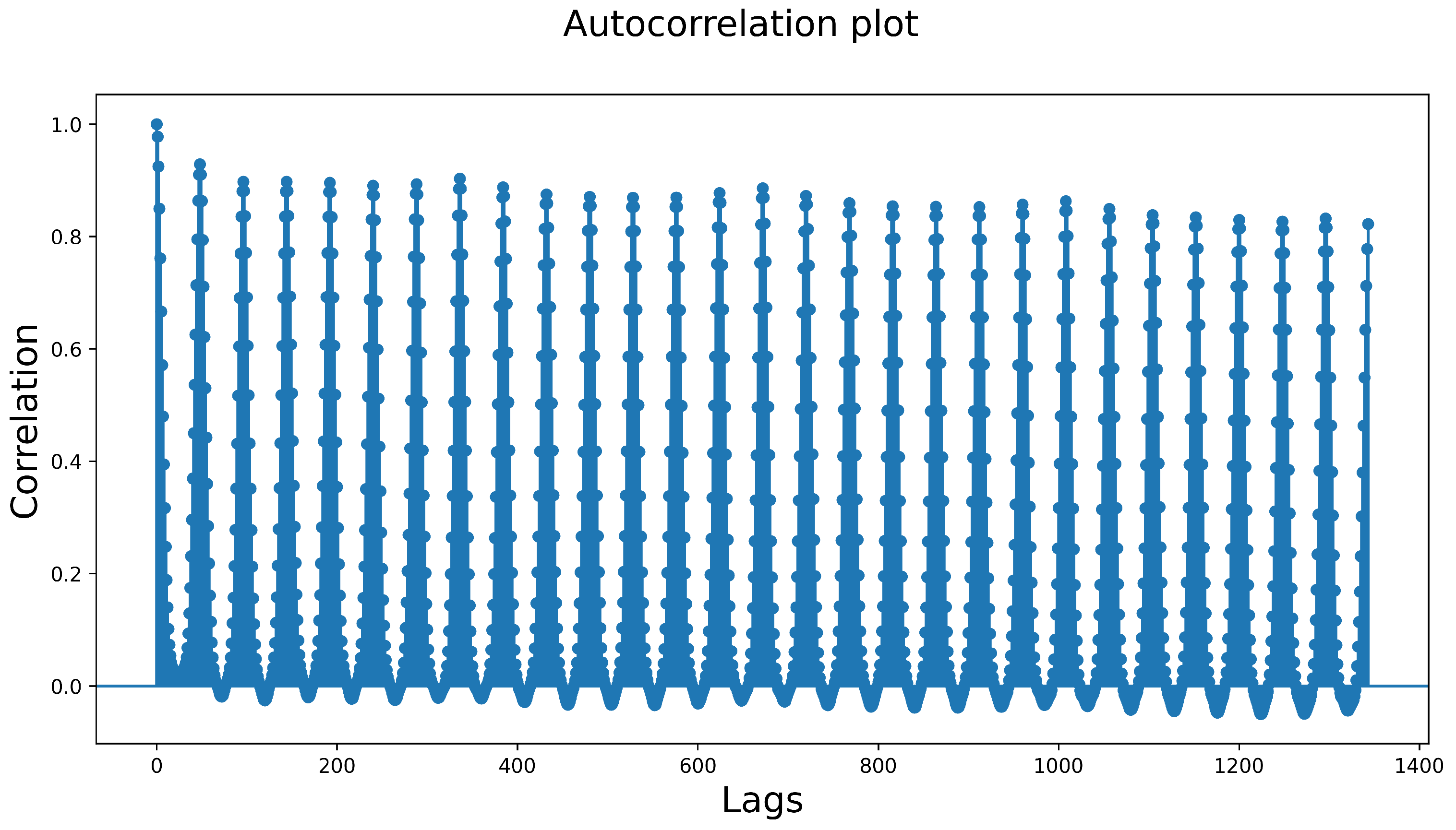
Once the best models, features and hyperparameter values were selected, the models were retrained using all the available data to generate the final solution. For instance, for week 1 (from 16 October 2018 to 22 October 2018), each of the models was evaluated in four weeks, ranging from 25 September 2018 to 1 October 2018, 2 October 2018 to 8 October 2018 and 9 October 2018 to 15 October 2018, respectively, and the final forecasts were generated using all the historical data up to 15 October 2018 included. The number of weeks used for model selection was mainly determined from the autocorrelation plot for the demand historical data (see Figure 4). It was found that considering the last four weeks of data to fine-tune and validate the models offered a good compromise between having a robust test set and assessing the results against weeks with conditions comparable to the target week.
For the next stage, several battery schedules were designed using the combinations of the best performing models for each forecasting task. The raw scores obtained by these schedules, according to the objective function (2), are not accurate enough to control the quality or the stability of the solution: for instance, the score for summer days will in general be much higher than the score for winter days due to the high PV power generation achievable in summer. Instead, to better assess the proposed solution, for each challenge week, the score achieved by an optimal schedule designed with perfect information (i.e., actual values of demand and PV power generation) was computed for the four test weeks. Then, the proposed battery schedules were evaluated according to the ratio of the optimal achievable score to the one obtained for each solution, as explained in Section 3, and the final battery schedule was decided accordingly.
In a real-life scenario, the main goal is to develop the best possible battery schedule for the week ahead. Due to fluctuations in the climatic conditions and shifts in the trend of energy demand, even very accurate predictive models would benefit from some fine-tuning to forecast the next weeks PV power generation and demand. Small adjustments and variations made to the core solution in order to provide reliable schedules for the four target weeks are detailed for each specific task in the subsequent sections.
2.4. Photovoltaic (PV) Power Prediction
PV power forecasting can support the integration and optimal utilisation of solar power sources into distribution networks [13]. However, due to the volatility and stochastic nature of solar energy, which depends on weather and atmospheric conditions such as the level of clouds and coverage, making predictions of PV power generated by solar energy sources is extremely challenging. Several methods for the prediction of PV power have been proposed in the literature, including physical models, statistical models, and machine learning models [13,14,15]. The performance of these methods depends on the precise task, the available data as well as the data resolution and prediction window. Typically, the forecasts are obtained using a number of external sources including solar irradiance, wind, humidity and atmospheric pressure [14,26]. Sky-image-based techniques have been employed for time horizons of under one hour, while satellite-image-based techniques were found to be more suitable for the prediction of several hours ahead [27].
Methods based on statistics and machine learning have been applied for short- and long-term predictions. In addition, many studies only focus on the prediction of solar irradiance, since it is highly correlated to PV power. A detailed review of these methods can be found in [26] which also provides guidance on the suitability of different methods depending on the time horizon and the prediction window.
2.5. Models
In this study, three main methods for PV forecasting were chosen and compared, including random forest (RF) and deep learning methods based on long short time memory (LSTM) and convolutional neural networks (CNNs).
2.5.1. Random Forest
The Random Forest (RF) method is a well-established ensemble learning technique which is widely used for classification and regression problems. Originally developed by Breiman [28], it builds weak learners on bootstrap samples using a random subset of variables to increase prediction accuracy and reduce bias by averaging results across multiple trees. This approach overcomes the limitations of decision trees methods based on single classifiers, which tend to have low accuracy and instability due to high sensitivity to small changes in the datasets. In the literature, RF has been successfully applied to the prediction of PV generation [29], and it has been chosen in this study due to the ease of use and good predictive performance. During initial experiments, RF was preferred over gradient boosting because it was less prone to overfitting. The RF was trained using the same validation strategy explained in Section 2.3 and hyperparameters (the minimum number of observations per leaf, number of trees and maximum number of splits) were optimised using the Bayesian optimisation approach [30]. Temperature data from locations 5 and 6 were removed, while irradiance data from all remote locations were kept. Furthermore, from test week 2, a cyclic feature for indicating the time of the day and month was included (see Section 2.6.1 below). Finally, the temperature was smoothed by taking a moving average of the two previous and the current time steps to take into account the possible delayed effect of the temperature. The complete available historical data were used for training in all weeks except for week 4, where only the last year of data was considered. This was due to the fact that, as the training data size became bigger, the prediction performance of the model started to decrease in addition to an increase in the time taken to train.
2.5.2. LSTM and CNN-LSTM
LSTM models are a type of recurrent neural network that have been demonstrated to perform exceptionally at time series forecasting in recent years, and are a common approach to weather and PV generation prediction [13,15]. The LSTM architecture includes a mechanism that can forget unimportant features during the learning process, while retaining information of long-term dependencies. This means that both short-term daily dependencies between irradiance, temperature, and power output can be learned, as well as the long-term trends such as seasonal variations. A sequence-to-ones LSTM approach was used to predict PV power with hyperparameters optimised using a grid search approach. While the optimal values of the various hyperparameters vary for each task, a common finding was that an LSTM depth of 3 with the number of hidden units set to 200, 400, and 600, and a moving window size of 96 time-steps (48 h) usually gave the best results.
In addition to the LSTM architecture, a CNN-LSTM was also compared at predicting PV generation. A CNN-LSTM model uses the same aforementioned principles as the LSTM with the addition of a front end CNN layer to carry out feature extraction before the LSTM input layer. The reasoning for this additional layer was to combine the LSTM’s superior temporal learning capabilities with the spatial learning capabilities of the CNN. This approach was implemented in an attempt to address the spatial challenges of the dataset, in that the model should learn the local relationships between the weather at the six locations at each individual time-step and use this to better predict the relationships with the PV data at the site. For all CNN-LSTM experiments, a single convolution layer followed by batch normalisation and ReLU activation was used to the perform front-end feature extraction.
Some additional data cleaning steps were implemented for CNN-LSTM and LSTM experiments. All data were normalised prior to training, and temperature data from locations 5 and 6 were removed, as well as irradiance data from location 4. For the days where any data were missing, the entire day of data was removed. In post-processing, all predicted values for PV power between sunset and sunrise were also set to 0. A notable difference between the two models was that the optimal value for the moving window size was found to be smaller for the CNN-LSTM at 76 time-steps (38 h), compared to 96 time-steps (48 h) for the LSTM.
Model Comparison
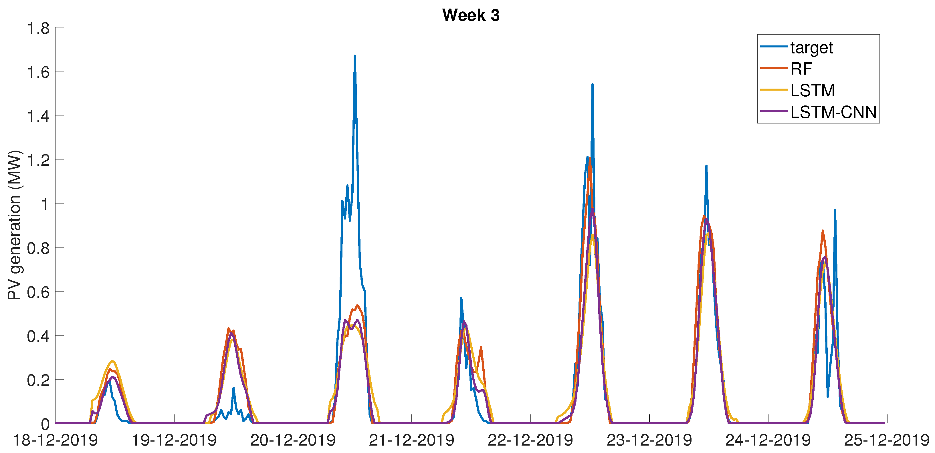
The models’ performance, in terms of MSE and , for the PV power prediction task across the four weeks is shown in Table 2. A comparable performance was obtained with the different models, with variations depending on the specific weeks. In terms of , RF was the best performing model for weeks 2 and 3, while the LSTM-based models were better in weeks 1 and 4. Overall, RF had larger variations in performance while the LSTM-based models seemed to be more consistent. The LSTM and CNN-LSTM methods produced similar results when comparing using MSE and , however, the CNN-LSTM proved to be more robust/consistent when repeating experiments. Figure 5 shows a comparison of the three models for week 1. It can be noticed that LSTM gave the ’smoothest’ results, whereas the CNN-LSTM performed better at predicting peaks or drops in PV power output at different times of day. A significant challenge that was faced throughout the development of the PV power forecasting models was that all tested models would consistently under-predict days with the highest power output, while over-predicting days with a low output. This is likely due to the fact that irradiance measurements were collected at geographically spread locations, which prevented the models from capturing the exact trend of the solar irradiance at the site under consideration. Furthermore, as shown in Table 2, it was found that the prediction task was less accurate in winter (week 3). This can also be seen in Figure 6. Sensitivity studies showed that further improvement of the accuracy of the model would not lead to the significant improvement of the challenge score, hence it was decided that these models were adequate for the optimisation task.
2.6. Demand Prediction
Electric load forecasting is a central task for electrical utilities. It plays a key role in power systems scheduling and maintenance, financial planning and energy trading, among others. This has motivated a wealth of research in this field, especially on the problem of forecasting load in the short-time horizon (see [7,11,12]). A wide variety of methods have been proposed and shown to be successful for different contexts and datasets. These approaches range from statistical techniques, such as multiple linear regression and ARIMA models to black-box models, including artificial neural networks and deep recurrent neural networks passing through general purpose regression algorithms such as gradient boosting machines and Gaussian process regression [6,31,32,33,34,35,36]. As it is sharply pointed out in [12] there is, as of yet, no single method that would consistently outperform every other technique for the short-time load forecasting problem. Rather, the choice of the most suitable techniques depends on the specific dataset, the forecast time horizon and factors such as the type of climate and of loads at the location where the data are collected.
In the case study at hand, some of the main challenges identified are the presence of unusual events (such as the 2018 FIFA World Cup and the 2020 lockdown) and the uncertainty introduced by the weather variables (see Section 2.4). Since the accuracy in demand prediction is critical for the quality of the battery schedule (as evaluated by the objective function (2)), most of the techniques mentioned above were tested, with the addition of the recently proposed TabNet model [37], according to the validation strategy described in Section 2.3. As a result of these tests, it was decided to use the top three models, which displayed similar performance: a CatBoost regressor model, an Artificial Neural Network (ANN) and a TabNet model. They are described in detail in Section 2.6.2.
2.6.1. Feature Engineering and Selection
The initial dataset, consisting of historical demand data and weather reanalysis data, was considerably augmented by engineering features. The added variables can be roughly classified into three groups: classical time series analysis features, time-related features and task-specific features.
- Time series analysis: Rolling statistics (both exponential and regular moving average and standard deviation of the demand for the previous week), lagged effects (demand value at the same hour for the past week) and trends at different scales (first order differences of temperature and solar irradiance and their averages over periods of 2, 12 and 24 h).
- Time-related: Hour of the day, day of the week, day of the month, month, year. Cyclic versions of hour of the day, day of the month and month consist of encoding these features as points in a 2D circle (see [32]).
- Task-specific: Bank holidays are labelled as Sunday and all features mentioned in the time-series analysis were shifted accordingly so that they coincided with the previous Sunday. Specific flags were added to distinguish the lockdown from regular days and to mark large sports events, such as England matches in the FIFA World Cup 2018.
This resulted in a dataset containing approximately 100 features. The SHAP module [38] was applied to the CatBoost model to reduce dataset dimensionality, keeping the 40 most important features. These include the exponential and regular moving average, lagged demand for the past week at the same hour, most of time-related features, both in regular and cyclic form and several averages of solar irradiance and temperature at different time windows.
2.6.2. Models
The regression models employed were trained to predict the average half-hourly demand value one week ahead. Although in the present scenario, the demand forecasting is only relevant during evening hours (see Appendix A), it was found that the models performed better when exposed to the whole dataset and trained to predict demand values for both day and evening hours. In order to obtain more accurate predictions for the evening hours, a weight was assigned to the samples corresponding to these hours and the models were fit to minimise the weighted mean squared error. The value of the weight was set using grid search in a set of powers of 10 ({1, 10, 100, 1000, 10,000}).
2.6.3. CatBoost
CatBoost [39] is an implementation of gradient boosting on decision trees developed by Yandex, which consistently achieves state-of-the-art performance in several practical tasks and is often employed by top solutions in Kaggle competitions. Gradient boosting is an ensemble method that iteratively improves base predictors (the case of CatBoost, decision trees) by performing gradient descent greedily in a certain functional space [40].
In general, the default values were used in the model except for a few hyperparameters that prevent overfitting or control the complexity of the model. Concretely, the following hyperparameters were defined according to a grid search around initial sensible values obtained by manual experimentation: n_estimators (maximum number of trees), depth (which controls the size of each decision tree), max_bin (the number of splits for numerical features) and rsm (the proportion of the features considered for each split).
2.6.4. Artificial Neural Network
Artificial neural networks are a type of machine learning model loosely inspired by the structure of biological neural networks. These models consist of a directed graph organised into layers whose nodes are connected to the nodes of the next layers. There are two distinguished layers, the input layer which receives the data and the output layer which is expected to yield the desired values. The remaining layers are known as hidden layers. Each layer is composed of several nodes, called neurons, which receive values from nodes on the previous layer (or the initial data in the case of the input layer), generate a new value applying a certain function to the inputs, and then passes it to all neurons in the next layer.
To prevent multicollinearity issues, several features are discarded. In particular, only cyclic versions of time-related features are included, the temperature and solar irradiance are removed for all but the two most uncorrelated locations. The architecture of the final artificial neural network used is composed of three hidden fully connected layers, with 64, 32 and 16 neurons, respectively. To define these architectures, the total number of hidden neurons was set to be proportional to the degrees of freedom of the problem (i.e., number of samples in training set divided by number of features) and the progressive reduction by factors of two in each layer was decided a priori. Having fixed these parameters, the number of hidden layers and neurons in the first hidden layer were selected using grid search. The ReLu activation was applied for all layers, and the Adam optimiser was used with the default learning rate 0.001.
2.6.5. TabNet
TabNet [37] is a novel deep neural network architecture specially designed for handling tabular data that reportedly outperform or is on par with standard neural network and decision tree variants. This new architecture learns directly from the raw numerical (not normalised) features, by employing batch normalisation layers and dedicated feature transformers blocks. One of its main novelties consists of the combined use of attention mechanism and a learnable mask to achieve instance-wise feature selection. Additionally, the learned weights in these layers can be used to interpret the outputs of the model, offering at the same time in-built feature selection and interpretability.
Similarly as in the case of the artificial neural network, the non-cyclic versions of time-related features and the temperature and solar irradiance for most locations were removed. Regarding the hyperparameters, using grid search, the value of width and steps were set, which control, respectively, the number of hidden neuron and hidden blocks. The ranges for the grid search were determined following [37] (guidelines for hyperparameters).
2.7. Model Comparison
The quality of the models was mainly evaluated according to the average MSE and errors attained in the validation sets, that is, in the four weeks prior to the target week. In general, while CatBoost is the strongest model by a slight margin, the three models attained a similar performance in validation and considerably beat the naive baseline of repeating the previous week demand values (see Table 3 below). In addition, the models’ predictions are sufficiently uncorrelated to obtain both variance and bias reduction by averaging their outputs.
The performance was relatively stable across different seasons. Figure 7 and Figure 8 display the forecast and actual demand for an autumn and a winter week, respectively. The few relatively large errors that can be appreciated in the plots correspond to day hours, which was to be expected from the choice of the loss metric for the models’ training.
The demand values for week 4, corresponding to the lockdown, are difficult to forecast, especially due to the less regular consumption patterns observed during this period, a fact that is reflected in the relatively low performance of the baseline model. It was found that reducing the size of the training set to only one year worked best for this task, as opposed to using the whole dataset to fit the models. Intuitively, this reduction helps the models assign similar importance to the energy consumption patterns from regular and lockdown times.
2.8. Optimisation
The deterministic version of the optimisation problem that results from using the forecast values of demand and PV power as parameters can be formulated as a program with a linear objective function and at most quadratic constraints. Thus, it falls in the class of second-order cone programs, which can be effectively solved using both commercial and free (for academic purposes) software. In the present work, the SCIP Optimisation Suite [41] was employed as a solver, which efficiently finds optimal or close-to-optimal solutions to the problem by using interior point methods [42] combined with heuristics to speed up the convergence. For more details on the modelling of the optimisation problem, the reader is referred to Appendix A.
2.9. Battery Charge Smoothing
This section concludes by detailing how the battery schedule is designed from the predictions for future demand and PV generation.
As already stated, the forecast values are used as parameters of a deterministic optimisation problem. Not surprisingly, it was found that this naive strategy led to the design of far from optimal battery schedules, mainly due to the volatility of the PV power generation. For this reason, the following post-processing step was applied to the output of the optimiser. Let and be, respectively, the total charge of the battery prescribed by the optimiser and the total predicted PV power generation (in MW), and let . The battery schedule is modified so that, for each day hour h, the charge is set to , where is the prediction for the PV power generated at time h measured in MW (see Appendix A for the notation). A common ratio r is chosen for each hour because the distribution of the percentage errors of the models for the PV power prediction did not considerably vary across the different hours. This modification allows to split evenly during the day the total charge prescribed by the optimiser, which intuitively counteracts the point estimation errors incurred by the model. The effectiveness of this technique was experimentally verified (see Section 3).
Finally, with the aim of improving the quality of the battery schedule and reducing the variance, the best way of combining the outputs from each model for the demand and the PV power was evaluated in the validation sets. Since there were at most three different models for each task, only the different possible combination of averages of the predictions were tested.
3. Results
In this section, the results obtained for the four challenge weeks referred at the beginning of Section 2 were analysed. The main criterion to evaluate the quality of the battery schedules proposed for these weeks is the score assigned by the objective function (2).
As explained in Section 2.3, in order to compare the performance across different weeks, the scores were normalised by computing the ratio between the optimal achievable score with the perfect information of the demand and PV power generation and the score of the proposed solution. More concretely, a quantity called Score ratio to evaluate the solutions is computed as follows:
The score of a battery schedule can be decomposed as a product of two factors, one linked to the evening peak reduction and another related to the amount of solar energy used. To understand the impact of the forecasting errors in the quality of the solutions, for each week the demand ratio and the PV ratio scores, computed in an analogous way to Equation (3), were also assessed. The final results are summarised in Table 4 below. Except for week 2, the performance was stable and in the range of 87–89%, which was consistent with the results observed in the validation sets and represents on average an improvement of up to 10% over the naive baseline solution.
The disaggregation of the scores clearly shows that the accuracy in the demand prediction is critical to the quality of the battery schedule. On the other hand, the proposed charging pattern of the battery is generally able to use the PV power generated almost optimally. As an example, this characteristic can be appreciated for the schedule corresponding to week 4 in Figure 9.
Regarding week 2, the solution was generated based only on the CatBoost model. As Figure 10 reveals, the predictions were off by a relatively large margin at the beginning of evenings on 14 March 2019 and 15 March 2019 (in addition to some large errors for day hours due to the metric choice as in Figure 7 and Figure 8). In turn, a single error of relatively high magnitude during the evening is heavily penalised by the objective function. The reason is that such single point errors result in a battery schedule that not only misses its target by a considerable margin at that point, but also conspires against the optimality of the distribution of the charge across the evening. This was corrected in the subsequent tasks by implementing two measures. In the first place, since the errors were likely due to overfitting, the performance and variance of all the possible averaged outputs of the three models (that is, the averages of pairs of models and the average of the three models) were assessed in the validation set to decide the best forecast. The second measure consisted of considering a new metric with validation purposes that could detect big single point errors. Concretely, the difference between the maximum and the average error incurred by each proposed forecast was computed to control that point errors were approximately evenly distributed across the evening hours.
4. Discussion
In this section, some possible paths to further improve the three critical tasks involved in the battery schedule design are discussed, namely PV generation forecasting, demand prediction and optimisation strategy.
A significant challenge faced in predicting PV generation was that in some weeks, there were large variations between the irradiance measurements at the various locations. Additionally, high irradiance readings at the six weather locations did not necessarily result in high irradiance readings at the PV site and vice versa. This can be seen in Figure 11. The top part of the plot shows the prediction of PV power for week 1, while the bottom part shows the irradiance at the different locations obtained from the weather data. It can be seen from the plots that inaccurate PV power predictions are typically caused by large variations between irradiance at the location of the solar panel (which is not available for the prediction task) and the measured irradiance at the other geographically spread locations obtained from the weather data. Although this is addressed by selecting machine learning architectures that typically perform well at inferring these complex spatial and temporal relationships, the scope of the challenge meant that less focus was placed on PV power prediction compared to other areas, leaving room to improve these models further. An example could be to experiment with different methods of geostatistical interpolation when re-sampling weather data from hourly to half-hourly time steps. Another possible improvement could be to include physical models that describe how PV power generation varies as a function of the temperature of the panel.
Regarding the demand prediction, it was discovered that the combination of MSE and as metrics to evaluate the fitness of a forecast was not entirely appropriate. As verified for week 2, these metrics fail to capture some large point estimation errors that lead to poor battery schedules in terms of peak demand shaving. In consequence, a promising path to improve the quality of the battery schedules consists of using of a loss metric that is directly related to the objective function to train the demand predictive models. On another note, the prediction of demand during exceptional periods such as the lockdown poses a challenge of independent interest. More refined approaches than the one adopted in this work could be applied to give a more systematic solution in such situations. In particular, applying transfer learning techniques seems a promising path.
Finally, different general techniques to tackle constrained optimisation problems under uncertainty could be applied for this problem. For instance, an end-to-end training approach, where the optimal battery schedule is learnt directly from the historical data without the need for the intermediate forecasting of demand and PV power generation might be interesting for this problem. We refer to [43] for a discussion on other possible approaches to optimisation problems under uncertainty and the exposition of a novel technique based on fitting probabilistic models to data according to a task-based loss.
5. Conclusions
In this paper, an end-to-end solution is proposed to the problem of designing an optimal battery schedule according to a natural criterion of combining evening peak shaving and the maximisation of solar energy usage from historical data. The precise formulation of the corresponding constrained optimisation problem was defined by ESC and WPD in a recent Data Science Challenge aimed at demonstrating the value that can be engineered from the data.
A two-stage approach is taken, consisting of fitting predictive models to data and then solving a deterministic optimisation problem using the forecast values as parameters. To this end, well-known machine learning algorithms, both specific and general purpose, convex optimisation and task-specific processing techniques are employed.
For the first part, several machine learning models to forecast PV power generation and demand are evaluated. The models for PV generation forecasting showed variation in performance across different testing weeks, hence highlighting the importance of developing a robust validation strategy for model selection, while CatBoost showed consistent performance for demand forecasting. Finally, an ad hoc optimisation strategy that uses both the prediction from machine learning models and the output of the optimiser to devise an optimal battery schedule is presented to find the optimal battery schedule. This strategy involves the fine tuning and validation of the predictive models in order to maximise a non-standard metric, namely the score of the resulting battery schedule.
Despite the high level of uncertainty inherent to PV power generation and demand, accentuated by the relatively long required forecasting period (one week ahead) and the COVID-19 pandemic, the overall performance obtained demonstrates the potential to generate value from the data in an idealised version of the battery schedule problem. Indeed, it was shown that the proposed approach can improve by up to 10% simpler solutions and reach close to 90% of the value of the ideal optimal solution with perfect information of the future.
The simplifications made when formulating the optimisation model constitute the main limitation of this work. For instance, the model does not take into account the degradation of the battery and it restricts the discharging/charging patterns to fixed time windows. These assumptions were adopted by the Data Science Challenge. The problem solved is hence an idealised version of the real challenges faced by the distribution network operators. It would be interesting to enrich the model by considering some relevant realistic restrictions, such as battery degradation, round-trip efficiency and the cost of electricity to test the scalability of the described solution. Other conceptual frameworks to approach this problem, such as stochastic optimisation, task-based optimisation or end-to-end learning, should be considered in future work. Among them, stochastic optimisation has the potential of leading to a provable robust design of battery schedules through the accurate estimation of the probability distributions for demand and PV power generation.
Author Contributions
Conceptualisation, E.B., C.G., J.F. and G.T.; methodology: optimisation, E.B., machine learning, E.B., C.G. and J.F.; software, E.B., C.G. and J.F.; validation of optimisation strategy, E.B.; writing—original draft preparation, E.B., C.G., J.F. and G.T.; writing—review and editing, G.T.; funding acquisition, C.G. and G.T. All authors have read and agreed to the published version of the manuscript.
Funding
C. Giannetti and E. Borghini are supported by the UK Engineering and Physical Sciences Research Council (EPSRC) project EP/S001387/1. G. Todeschini is supported by the EPSRC project EP/T013206/1. J. Flynn is supported by the M2A funding from the European Social Fund via the Welsh Government (c80816), the Engineering and Physical Sciences Research Council (Grant Ref: EP/L015099/1). We further acknowledge the support of the Supercomputing Wales project (c80898 and c80900), which is partly funded by the European Regional Development Fund (ERDF) via the Welsh Government. All authors would like to acknowledge the support of the IMPACT project, part-funded by the European Regional Development Fund (ERDF) via the Welsh Government.
Institutional Review Board Statement
Not applicable.
Informed Consent Statement
Not applicable.
Data Availability Statement
The datasets are publicly available at the Western Power Distribution Open Data Hub site (https://www.westernpower.co.uk/innovation/pod, accessed on 1 May 2021) upon login. The code required to generate the results referred in the article will be made publicly available, but will also be shared upon request before publication.
Acknowledgments
The authors would like to thank Stephen Haben and the organiser team of the ‘Presumed Open Data: Data Science Challenge’ and Alma Rahat for useful discussion and suggestions concerning the methodology and machine learning approaches.
Conflicts of Interest
The authors declare no conflict of interest.
Appendix A. Modelling of the Optimisation Problem
In this appendix, the formal definition of the constrained optimisation problem is given. As already mentioned, the overarching goal was to design an optimal battery schedule for each day d in the following week, which will have the same time resolution as the dataset. Thus, there are 48 decision variables for each day d, which represent the charge/discharge of the battery in MW. In what follows, the day will be fixed and the subscript d dropped, since the battery schedules for different days are independent in the model. The (unknown) parameters for the model are the load and the PV power generated , both averaged over half-hour intervals and measured in MW. For convenience, two additional sets of variables are introduced: and . The first set models the effective amount of solar energy used by the battery schedule (that is, for ), while the second set accounts for the state-of-energy of the battery at each step. It is defined as , where the coefficient converts power (MW) into energy (MWh).
Appendix A.1. Constraints
Some restrictions on the schedule are imposed to model physical limitations on the operation of the battery, such as maximum capacity and charge or discharge rate limits. It should be remarked, however, that for the sake of simplicity, the modelling disregards the battery degradation.
One of the main inconveniences of PV generation stems from the fact that it typically takes place during day time when power demand is relatively low, while demand peaks occur in the evening when there is little-to-no solar generation. To address this situation, the battery will be allowed to charge only during the ‘day hours’ (from 5:00 a.m. to 3:00 p.m.) and discharge during the “evening hours” (from 3:30 p.m. to 8:30 p.m.). Accordingly, the sets and are defined, where the indices represent one of the 48 half-hour periods in the day (thus, for instance, 11 corresponds to the half-hour period starting at 5 a.m.). The convention that when the battery is charging and negative otherwise is adopted. The complete set of constraints is as follows:
For the particular case study, the limits are , , , .
Appendix A.2. Objective Function
The objective function is composed of two factors, one related to peak shaving during the evening and the other to the storage of solar energy during the day hours. In order to formulate the peak shaving component, the parameter as is considered, which captures the peak of the demand during the evening without using any energy stored in the battery. The peak shaving factor will be simply the difference between this peak and the maximum demand experienced by the network if the use of the battery is allowed. More precisely, is computed from and as
(Recall that is by convention negative when the battery discharges.)
As for the maximisation of the use of energy generated by the PV panels, consider the variables:
which store, respectively, the total energy charged and the total amount of solar energy charged according to the battery schedule . In terms of these variables, the solar energy use associated factor is:
where is a user-defined parameter that ’rewards’ the use of solar energy according to some relevant criterion. In the present case, since the lifecycle GHG emission intensity of solar PV is estimated to be of the average lifecycle emission intensity of the grid in the UK, we set . Finally, the objective function J is simply the product of these two factors, that is:
Appendix A.3. Optimisation Model
The final optimisation problem obtained by assembling all the information from the previous subsections can be formulated formally as a second-order cone program (SOCP). This class of problems admits (often) effective solutions by means of interior point methods [42], and there are both dedicated commercial and free (for academic purposes) solvers.
Before presenting the final formulation of the optimisation problem as a SOCP, some manipulations with the objective function will need to be performed. This is mainly due to the fact that the objective function is not linear on the decision variables (it is not even polynomial). Notice in first place that depends quadratically on the variables and . At first sight, this does not look very promising because is not a linear function of the decision variables . However, is piecewise linear on the variables and a well-known trick (see for instance [44] (p. 66)) allows to handle this situation by adding a new constraint. Putting all together, the problem is formulated as:
Note that it is also necessary to add a constraint to force the variable to be strictly positive. Otherwise, setting all decision variables and the score variable S as an arbitrarily large number would be a feasible solution. Formally, this lower bound could be chosen as some value below the minimum total generation of PV power across the dataset. However, it was observed experimentally that optimal solutions often prescribe charging the battery to full capacity (even in winter), so usually a value at least half the maximum as lower bound for is chosen in the runs, which additionally speeds up the convergence to an optimal solution.
References
- Energy Trends: UK Renewables. Available online: https://www.gov.uk/government/statistics/energy-trends-section-6-renewables (accessed on 5 May 2021).
- Locatelli, G.; Palerma, E.; Mancini, M. Assessing the economics of large Energy Storage Plants with an optimisation methodology. Energy 2015, 83, 15–28. [Google Scholar] [CrossRef] [Green Version]
- Infield, D.; Freir, L. Renewable Energy in Power Systems; Wiley: Hoboken, NJ, USA, 2020. [Google Scholar]
- Beltran, H.; Perez, E.; Aparicio, N.; Rodriguez, P. Daily Solar Energy Estimation for Minimizing Energy Storage Requirements in PV Power Plants. IEEE Trans. Sustain. Energy 2013, 4, 474–481. [Google Scholar] [CrossRef] [Green Version]
- Mexis, I.; Todeschini, G. Battery Energy Storage Systems in the United Kingdom: A Review of Current State-of-the-Art and Future Applications. Energies 2020, 13, 3616. [Google Scholar] [CrossRef]
- Din, G.M.U.; Marnerides, A.K. Short term power load forecasting using Deep Neural Networks. In Proceedings of the 2017 International Conference on Computing, Networking and Communications (ICNC), Silicon Valley, CA, USA, 26–29 January 2017; pp. 594–598. [Google Scholar] [CrossRef] [Green Version]
- Gross, G.; Galiana, F. Short-term load forecasting. Proc. IEEE 1987, 75, 1558–1573. [Google Scholar] [CrossRef]
- Vu, D.H.; Muttaqi, K.M.; Agalgaonkar, A.P. Short-term load forecasting using regression based moving windows with adjustable window-sizes. In Proceedings of the 2014 IEEE Industry Application Society Annual Meeting, Vancouver, BC, Canada, 5–9 October 2014; pp. 1–8. [Google Scholar] [CrossRef] [Green Version]
- Sinden, G. Characteristics of the UK wind resource: Long-term patterns and relationship to electricity demand. Energy Policy 2007, 35, 112–127. [Google Scholar] [CrossRef]
- Staffell, I.; Pfenninger, S. The increasing impact of weather on electricity supply and demand. Energy 2018, 145, 65–78. [Google Scholar] [CrossRef]
- Hong, T. Short Term Electric Load Forecasting. Ph.D. Thesis, North Carolina State University, Raleigh, NC, USA, 2010. [Google Scholar]
- Hong, T.; Fan, S. Probabilistic electric load forecasting: A tutorial review. Int. J. Forecast. 2016, 32, 914–938. [Google Scholar] [CrossRef]
- Wang, K.; Qi, X.; Liu, H. Photovoltaic power forecasting based LSTM-Convolutional Network. Energy 2019, 189, 116225. [Google Scholar] [CrossRef]
- Sobri, S.; Koohi-Kamali, S.; Rahim, N.A. Solar photovoltaic generation forecasting methods: A review. Energy Convers. Manag. 2018, 156, 459–497. [Google Scholar] [CrossRef]
- Qing, X.; Niu, Y. Hourly day-ahead solar irradiance prediction using weather forecasts by LSTM. Energy 2018, 148, 461–468. [Google Scholar] [CrossRef]
- Shi, Y.; Xu, B.; Wang, D.; Zhang, B. Using Battery Storage for Peak Shaving and Frequency Regulation: Joint Optimization for Superlinear Gains. In Proceedings of the 2018 IEEE Power Energy Society General Meeting (PESGM), Portland, OR, USA, 5–9 August 2018; p. 1. [Google Scholar] [CrossRef] [Green Version]
- Silva, V.A.; Aoki, A.R.; Lambert-Torres, G. Optimal Day-Ahead Scheduling of Microgrids with Battery Energy Storage System. Energies 2020, 13, 5188. [Google Scholar] [CrossRef]
- Sossan, F.; Namor, E.; Cherkaoui, R.; Paolone, M. Achieving the Dispatchability of Distribution Feeders Through Prosumers Data Driven Forecasting and Model Predictive Control of Electrochemical Storage. IEEE Trans. Sustain. Energy 2016, 7, 1762–1777. [Google Scholar] [CrossRef] [Green Version]
- Wang, Z.; Negash, A.; Kirschen, D.S. Optimal scheduling of energy storage under forecast uncertainties. IET Gener. Transm. Distrib. 2017, 11, 4220–4226. [Google Scholar] [CrossRef]
- Scarabaggio, P.; Grammatico, S.; Carli, R.; Dotoli, M. Distributed Demand Side Management With Stochastic Wind Power Forecasting. IEEE Trans. Control Syst. Technol. 2021, 1–16. [Google Scholar] [CrossRef]
- Rigo-Mariani, R.; Chea Wae, S.O.; Mazzoni, S.; Romagnoli, A. Comparison of optimization frameworks for the design of a multi-energy microgrid. Appl. Energy 2020, 257, 113982. [Google Scholar] [CrossRef]
- Melhem, F.Y.; Grunder, O.; Hammoudan, Z.; Moubayed, N. Energy Management in Electrical Smart Grid Environment Using Robust Optimization Algorithm. IEEE Trans. Ind. Appl. 2018, 54, 2714–2726. [Google Scholar] [CrossRef]
- Hosseini, S.M.; Carli, R.; Dotoli, M. A Residential Demand-Side Management Strategy under Nonlinear Pricing Based on Robust Model Predictive Control. In Proceedings of the 2019 IEEE International Conference on Systems, Man and Cybernetics (SMC), Bari, Italy, 6–9 October 2019; pp. 3243–3248. [Google Scholar] [CrossRef]
- Presumed Open Data (POD). Available online: https://westernpower.co.uk/innovation/projects/presumed-open-data-pod (accessed on 1 May 2021).
- Western Power Distribution Open Data Hub Homepage. Available online: https://www.westernpower.co.uk/innovation/pod (accessed on 22 April 2021).
- Rajagukguk, R.A.; Ramadhan, R.A.A.; Lee, H.J. A Review on Deep Learning Models for Forecasting Time Series Data of Solar Irradiance and Photovoltaic Power. Energies 2020, 13, 6623. [Google Scholar] [CrossRef]
- Caldas, M.; Alonso-Suárez, R. Very short-term solar irradiance forecast using all-sky imaging and real-time irradiance measurements. Renew. Energy 2019, 143, 1643–1658. [Google Scholar] [CrossRef]
- Breiman, L. Random forests. Mach. Learn. 2001, 45, 5–32. [Google Scholar] [CrossRef] [Green Version]
- Antonanzas, J.; Osorio, N.; Escobar, R.; Urraca, R.; de Pison, F.M.; Antonanzas-Torres, F. Review of photovoltaic power forecasting. Sol. Energy 2016, 136, 78–111. [Google Scholar] [CrossRef]
- Snoek, J.; Larochelle, H.; Adams, R.P. Practical bayesian optimization of machine learning algorithms. In Advances in Neural Information Processing Systems; Curran Associates, Inc.: Red Hook, NY, USA, 2012; pp. 2951–2959. [Google Scholar]
- Hu, R.; Wen, S.; Zeng, Z.; Huang, T. A short-term power load forecasting model based on the generalized regression neural network with decreasing step fruit fly optimization algorithm. Neurocomputing 2017, 221, 24–31. [Google Scholar] [CrossRef]
- Moon, J.; Park, S.; Rho, S.; Hwang, E. A comparative analysis of artificial neural network architectures for building energy consumption forecasting. Int. J. Distrib. Sens. Netw. 2019, 15. [Google Scholar] [CrossRef] [Green Version]
- Park, D.; El-Sharkawi, M.; Marks, R.; Atlas, L.; Damborg, M. Electric load forecasting using an artificial neural network. IEEE Trans. Power Syst. 1991, 6, 442–449. [Google Scholar] [CrossRef] [Green Version]
- Lloyd, J.R. GEFCom2012 hierarchical load forecasting: Gradient boosting machines and Gaussian processes. Int. J. Forecast. 2014, 30, 369–374. [Google Scholar] [CrossRef] [Green Version]
- Singh, S.; Hussain, S.; Bazaz, M.A. Short term load forecasting using artificial neural network. In Proceedings of the 2017 Fourth International Conference on Image Information Processing (ICIIP), Shimla, India, 21–23 December 2017; pp. 1–5. [Google Scholar] [CrossRef]
- Hong, T.; Pinson, P.; Fan, S. Global Energy Forecasting Competition 2012. Int. J. Forecast. 2014, 30, 357–363. [Google Scholar] [CrossRef]
- Arik, S.Ö.; Pfister, T. TabNet: Attentive Interpretable Tabular Learning. arXiv 2019, arXiv:1908.07442. [Google Scholar]
- Lundberg, S.M.; Lee, S.I. A Unified Approach to Interpreting Model Predictions. In Advances in Neural Information Processing Systems 30; Guyon, I., Luxburg, U.V., Bengio, S., Wallach, H., Fergus, R., Vishwanathan, S., Garnett, R., Eds.; Curran Associates, Inc.: Nice, France, 2017; pp. 4765–4774. [Google Scholar]
- Prokhorenkova, L.; Gusev, G.; Vorobev, A.; Dorogush, A.V.; Gulin, A. CatBoost: Unbiased boosting with categorical features. In Advances in Neural Information Processing Systems; Bengio, S., Wallach, H., Larochelle, H., Grauman, K., Cesa-Bianchi, N., Garnett, R., Eds.; Curran Associates, Inc.: Nice, France, 2018; Volume 31. [Google Scholar]
- Friedman, J.H. Greedy function approximation: A gradient boosting machine. Ann. Stat. 2001, 29, 1189–1232. [Google Scholar] [CrossRef]
- Gamrath, G.; Anderson, D.; Bestuzheva, K.; Chen, W.K.; Eifler, L.; Gasse, M.; Gemander, P.; Gleixner, A.; Gottwald, L.; Halbig, K.; et al. The SCIP Optimization Suite 7.0; Technical Report; Optimization Online; Zuse Institute Berlin: Berlin, Germany, 2020. [Google Scholar]
- Potra, F.A.; Wright, S.J. Interior-point methods. J. Comput. Appl. Math. 2000, 124, 281–302. [Google Scholar] [CrossRef] [Green Version]
- Donti, P.L.; Kolter, J.Z.; Amos, B. Task-based End-to-end Model Learning in Stochastic Optimization. In Advances in Neural Information Processing Systems 30, Proceedings of the Annual Conference on Neural Information Processing Systems 2017, Long Beach, CA, USA, 4–9 December 2017; Guyon, I., von Luxburg, U., Bengio, S., Wallach, H.M., Fergus, R., Vishwanathan, S.V.N., Garnett, R., Eds.; Curran Associates, Inc.: Long Beach, CA, USA, 2017; pp. 5484–5494. [Google Scholar]
- Bisschop, J. AIMMS—Optimization Modeling; Lulu.com, 2006. Available online: https://documentation.aimms.com/_downloads/AIMMS_modeling.pdf (accessed on 8 June 2021).
Figure 1.
Illustration of the workflow of the proposed approach.

Figure 2.
Overview of the area considered for the study: the location of the substation, PV farms and four surrounding weather stations are shown. Map data ©2021 Google.
Figure 2.
Overview of the area considered for the study: the location of the substation, PV farms and four surrounding weather stations are shown. Map data ©2021 Google.

Figure 3.
Illustration of the walk-forward validation technique. The test sets, indicated in orange, represent the validation weeks.
Figure 3.
Illustration of the walk-forward validation technique. The test sets, indicated in orange, represent the validation weeks.

Figure 4.
The autocorrelation of the demand presents daily peaks, which steadily decrease as the lag increases (here, a lag unit represents a 30 min period). The plot displays the autocorrelation for a maximum lag of four weeks.
Figure 4.
The autocorrelation of the demand presents daily peaks, which steadily decrease as the lag increases (here, a lag unit represents a 30 min period). The plot displays the autocorrelation for a maximum lag of four weeks.

Figure 5.
Plots of model predictions for week 1 showing a comparison of the three proposed models with the target.
Figure 5.
Plots of model predictions for week 1 showing a comparison of the three proposed models with the target.

Figure 6.
Plots of model predictions for week 3. The prediction of PV power output is more challenging at low generation.
Figure 6.
Plots of model predictions for week 3. The prediction of PV power output is more challenging at low generation.

Figure 7.
Comparison between the prediction and the target for week 1. The ticks in the x axis correspond to midnight for each day.
Figure 7.
Comparison between the prediction and the target for week 1. The ticks in the x axis correspond to midnight for each day.

Figure 8.
Comparison between the prediction and the target for week 3. The special treatment for holidays leads to an accurate demand prediction for Christmas Eve.
Figure 8.
Comparison between the prediction and the target for week 3. The special treatment for holidays leads to an accurate demand prediction for Christmas Eve.

Figure 9.
Comparison between the battery charge pattern and the PV power generation for week 4. When the battery charge is greater than the PV power, the difference is taken from the grid.
Figure 9.
Comparison between the battery charge pattern and the PV power generation for week 4. When the battery charge is greater than the PV power, the difference is taken from the grid.

Figure 10.
Plot of Catboost model’s predictions for week 2. There are some large errors for the evenings of the fifth and sixth day.
Figure 10.
Plot of Catboost model’s predictions for week 2. There are some large errors for the evenings of the fifth and sixth day.

Figure 11.
The top plot shows the target and predicted PV power for week 1, while the bottom plot shows the irradiance measured at the location of the solar panel (which is not available for the prediction) and the irradiance obtained from the weather data at the other geographically spread locations (used in the prediction task).


Table 1.
Description of the variables and parameters used in the optimisation problem.
| Name | Meaning |
|---|---|
| Battery charge at time k in MW | |
| Energy load at time k in MW | |
| Minimum and maximum battery capacity in MW, resp. | |
| State-of-energy of battery at time k in MWh | |
| Minimum and maximum state-of-energy of battery in MWh, resp. | |
| PV power generation at time k in MW | |
| Sum of over all times k in a day | |
| Sum of over all times k in a day | |
| Coefficient that measures the environmental efficiency of PV power | |
| Auxiliary variable to store the new peak demand | |
| S | Auxiliary variable to store the score |
Table 2.
Comparison of three methods in predicting the PV power for the challenge weeks. The highest and lowest MSE for each week are highlighted in bold.
Table 2.
Comparison of three methods in predicting the PV power for the challenge weeks. The highest and lowest MSE for each week are highlighted in bold.
| Method | Week | MSE | |
|---|---|---|---|
| Random forest | 1 | 0.7625 | 0.2845 |
| Random forest | 2 | 0.8330 | 0.1125 |
| Random forest | 3 | 0.7168 | 0.0209 |
| Random forest | 4 | 0.8199 | 0.1806 |
| LSTM | 1 | 0.8323 | 0.1983 |
| LSTM | 2 | 0.8143 | 0.1060 |
| LSTM | 3 | 0.6948 | 0.0245 |
| LSTM | 4 | 0.8632 | 0.1610 |
| CNN-LSTM | 1 | 0.8539 | 0.1688 |
| CNN-LSTM | 2 | 0.8204 | 0.1077 |
| CNN-LSTM | 3 | 0.7140 | 0.0218 |
| CNN-LSTM | 4 | 0.8544 | 0.1535 |
Table 3.
Comparison of the three models for demand prediction in the four weeks. The highest and lowest MSE for each week are highlighted in bold.
Table 3.
Comparison of the three models for demand prediction in the four weeks. The highest and lowest MSE for each week are highlighted in bold.
| Method | Week | MSE | |
|---|---|---|---|
| CatBoost | 1 | 0.9222 | 0.0435 |
| CatBoost | 2 | 0.9695 | 0.0200 |
| CatBoost | 3 | 0.9690 | 0.0239 |
| CatBoost | 4 | 0.9443 | 0.0236 |
| ANN | 1 | 0.9264 | 0.0412 |
| ANN | 2 | 0.9306 | 0.0456 |
| ANN | 3 | 0.9678 | 0.0248 |
| ANN | 4 | 0.9305 | 0.0295 |
| TabNet | 1 | 0.8943 | 0.0592 |
| TabNet | 2 | 0.9120 | 0.0577 |
| TabNet | 3 | 0.9476 | 0.0403 |
| TabNet | 4 | 0.8815 | 0.0502 |
| Baseline | 1 | 0.7938 | 0.1154 |
| Baseline | 2 | 0.9043 | 0.0628 |
| Baseline | 3 | 0.9060 | 0.0724 |
| Baseline | 4 | 0.8370 | 0.0691 |
Table 4.
Scores obtained for each of the four weeks, expressed as a percentage of the optimal solution and disaggregated into demand- and PV power-related factors. For reference, the corresponding score obtained by copying the previous week demand and PV power are included.
Table 4.
Scores obtained for each of the four weeks, expressed as a percentage of the optimal solution and disaggregated into demand- and PV power-related factors. For reference, the corresponding score obtained by copying the previous week demand and PV power are included.
| Week | Avg. Demand Ratio | Avg. PV Ratio | Avg. Score Ratio | Baseline Score Ratio |
|---|---|---|---|---|
| 1 | 90.7135 | 97.5196 | 88.4466 | 82.3380 |
| 2 | 85.5383 | 95.7059 | 81.8722 | 79.0595 |
| 3 | 88.0555 | 99.0025 | 87.1435 | 76.5495 |
| 4 | 90.2056 | 97.8797 | 88.3836 | 80.4124 |
Publisher’s Note: MDPI stays neutral with regard to jurisdictional claims in published maps and institutional affiliations. |
© 2021 by the authors. Licensee MDPI, Basel, Switzerland. This article is an open access article distributed under the terms and conditions of the Creative Commons Attribution (CC BY) license (https://creativecommons.org/licenses/by/4.0/).
Share and Cite
MDPI and ACS Style
Borghini, E.; Giannetti, C.; Flynn, J.; Todeschini, G. Data-Driven Energy Storage Scheduling to Minimise Peak Demand on Distribution Systems with PV Generation. Energies 2021, 14, 3453. https://doi.org/10.3390/en14123453
AMA Style
Borghini E, Giannetti C, Flynn J, Todeschini G. Data-Driven Energy Storage Scheduling to Minimise Peak Demand on Distribution Systems with PV Generation. Energies. 2021; 14(12):3453. https://doi.org/10.3390/en14123453
Chicago/Turabian StyleBorghini, Eugenio, Cinzia Giannetti, James Flynn, and Grazia Todeschini. 2021. "Data-Driven Energy Storage Scheduling to Minimise Peak Demand on Distribution Systems with PV Generation" Energies 14, no. 12: 3453. https://doi.org/10.3390/en14123453
Note that from the first issue of 2016, this journal uses article numbers instead of page numbers. See further details here.