Sea Surface Temperature in Global Analyses: Gains from the Copernicus Imaging Microwave Radiometer

 , , , and
Abstract
:
1. Introduction
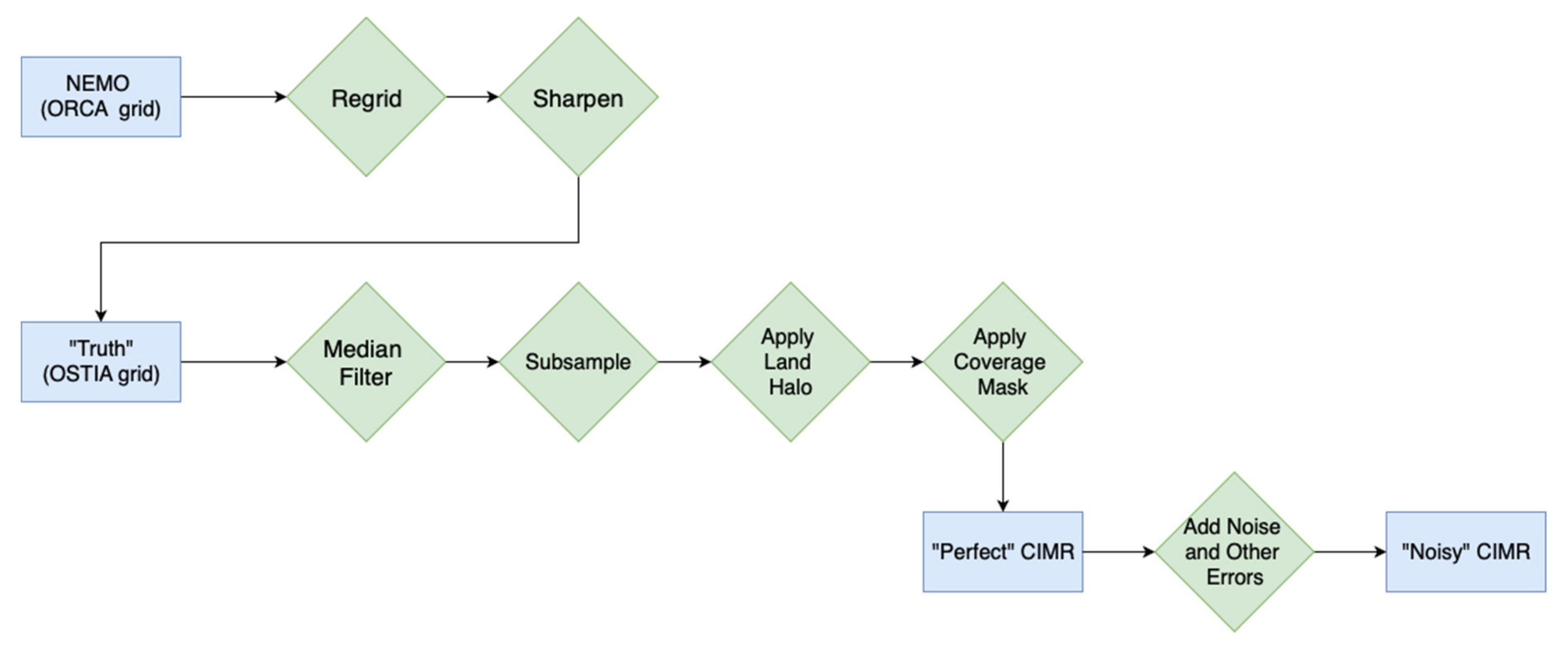
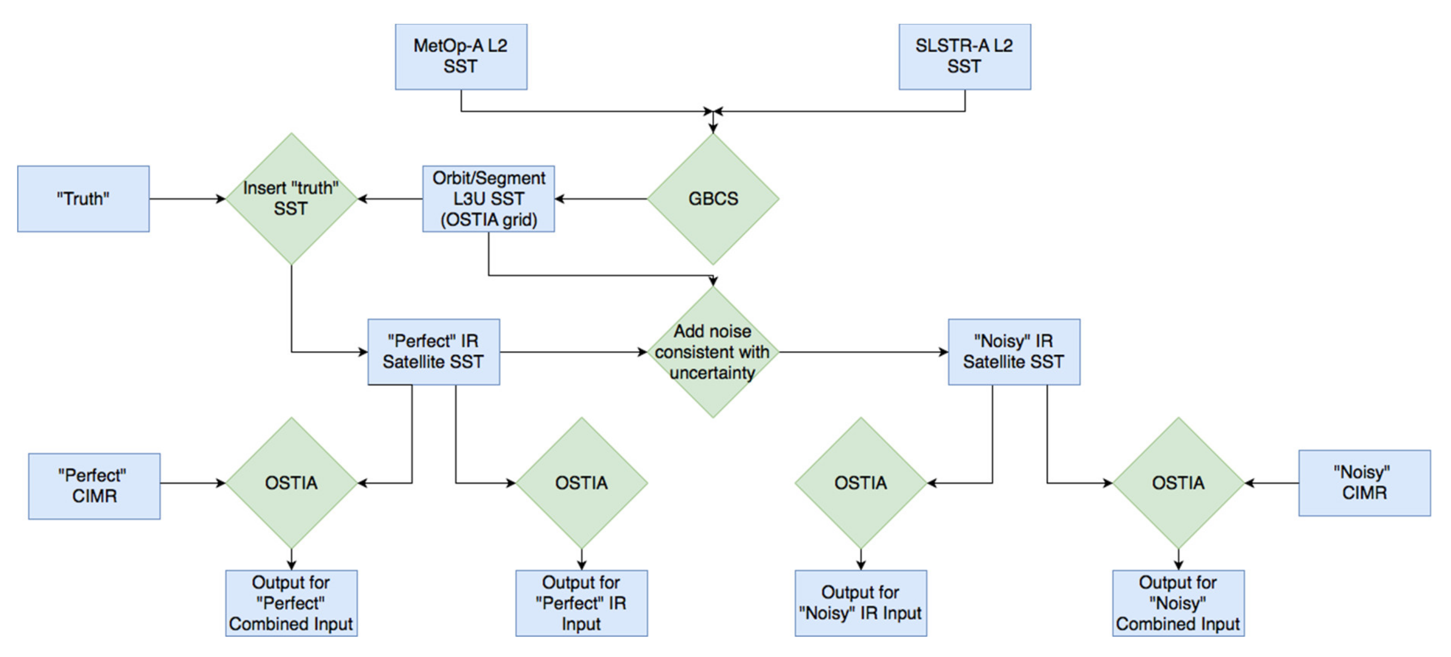
2. Methods
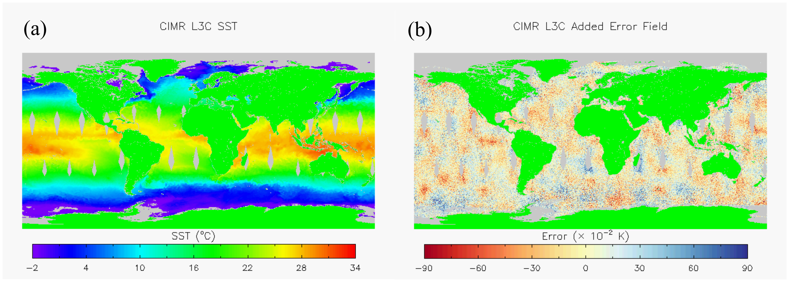
3. Results
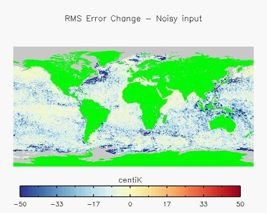
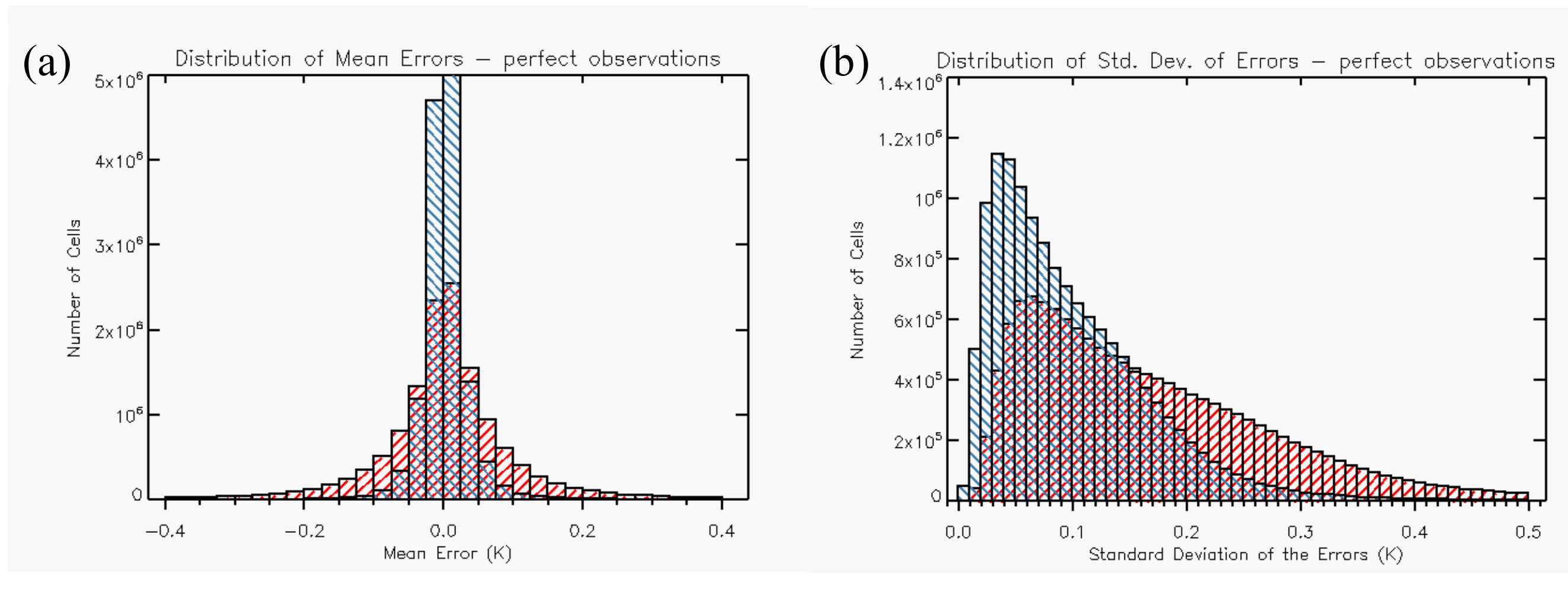
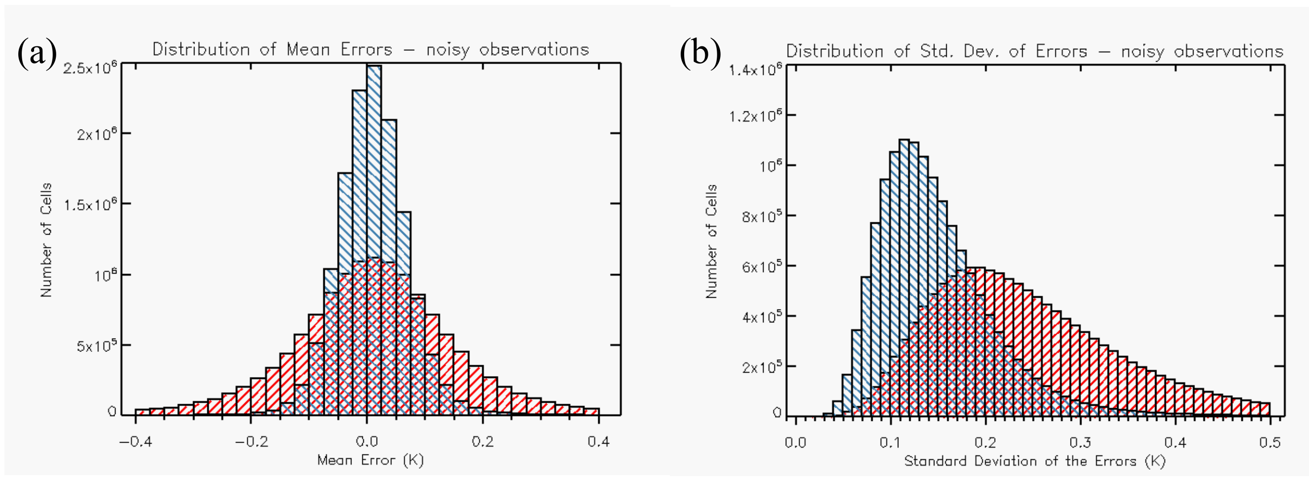
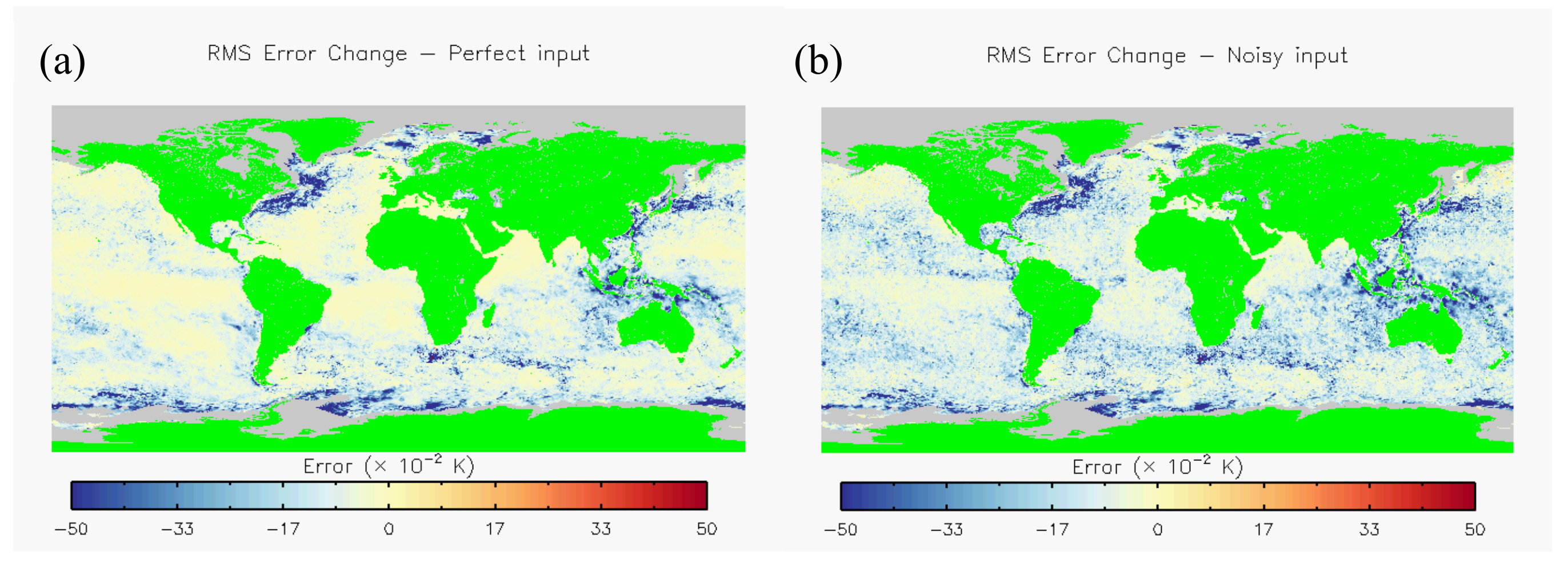
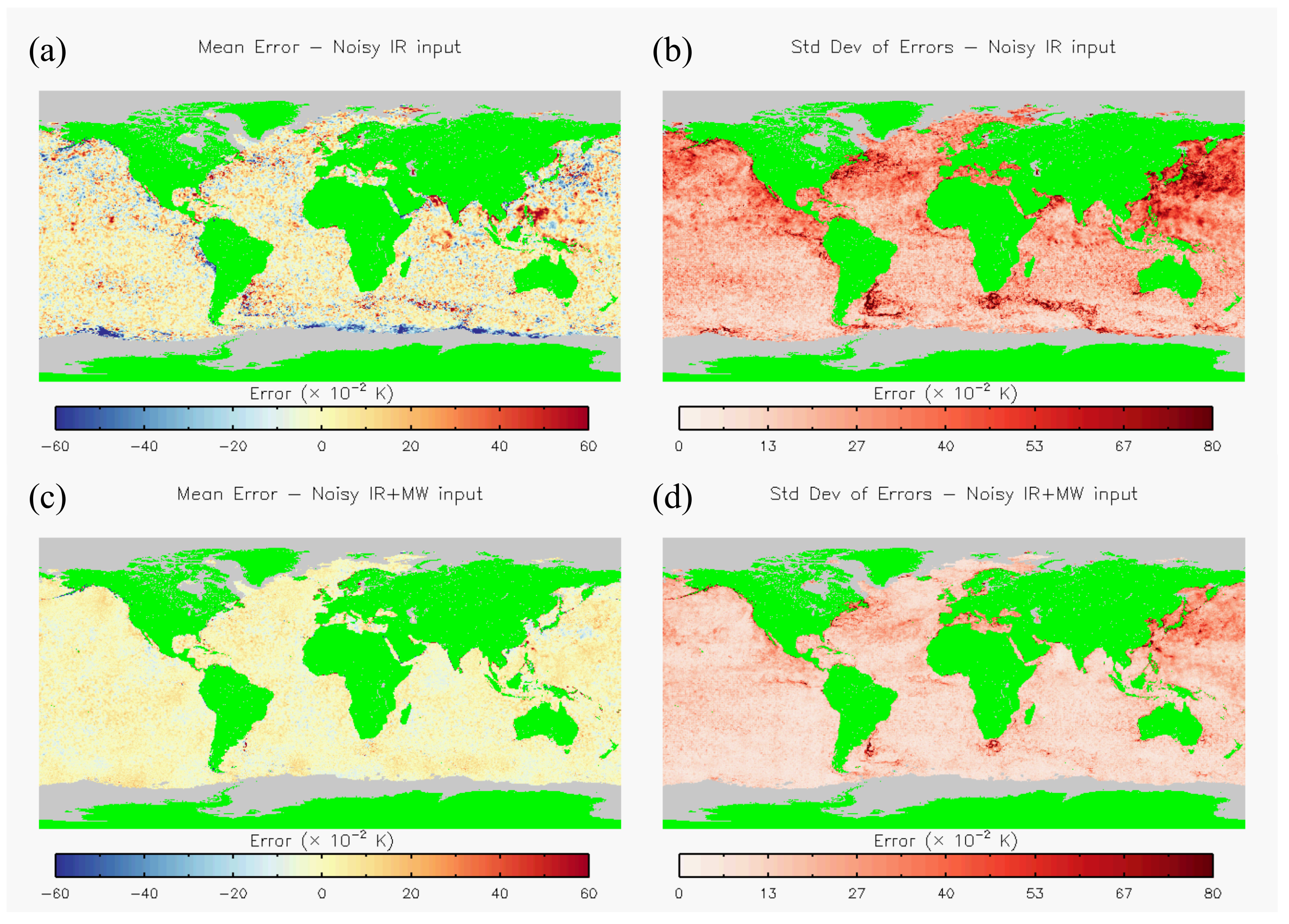
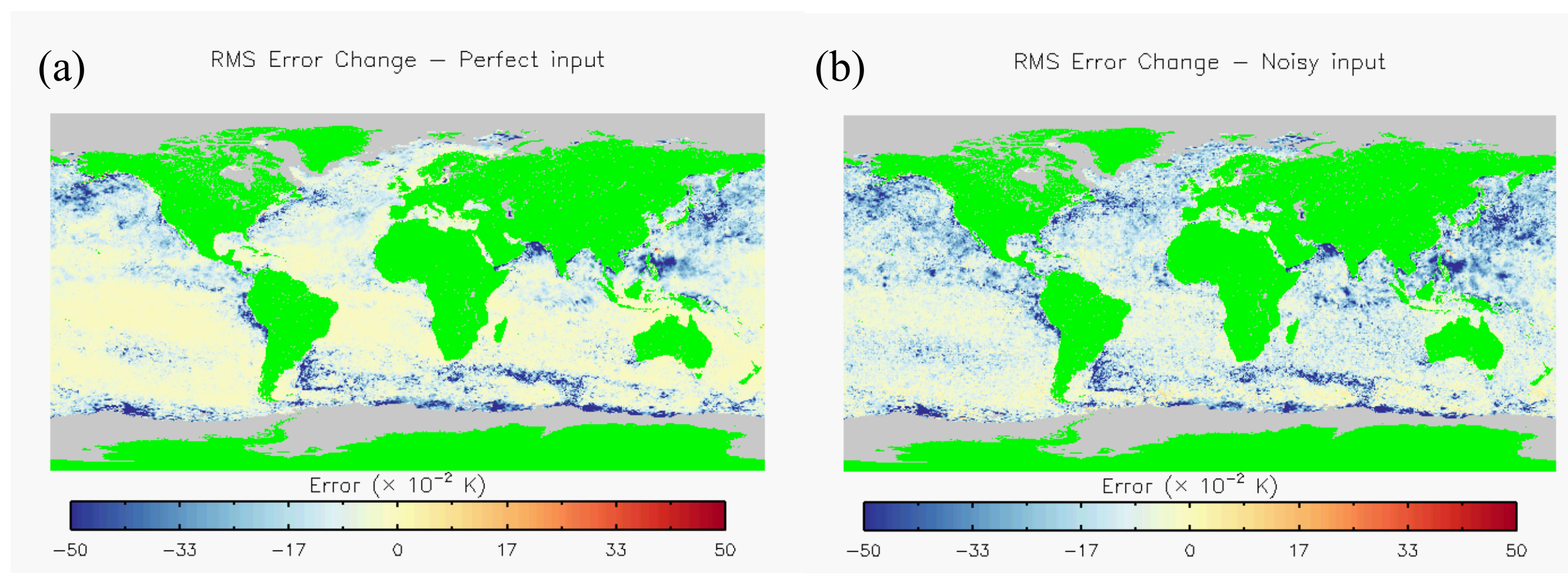
3.1. Error Statistics
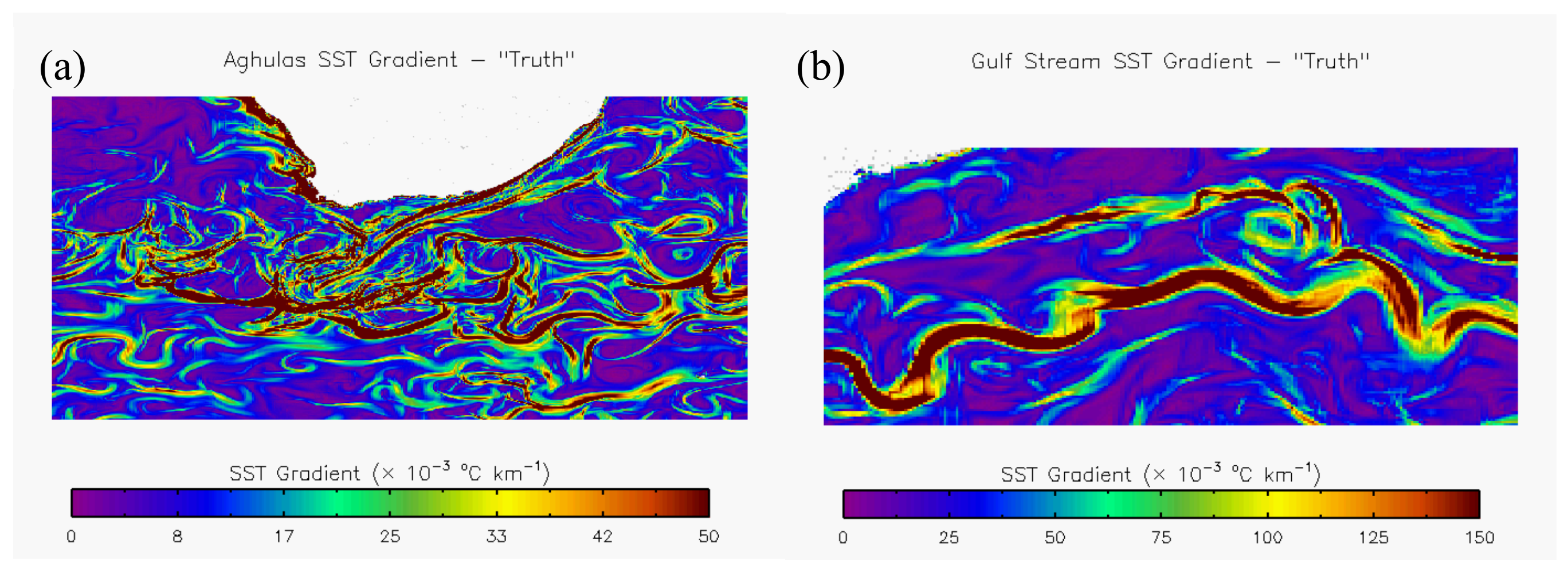
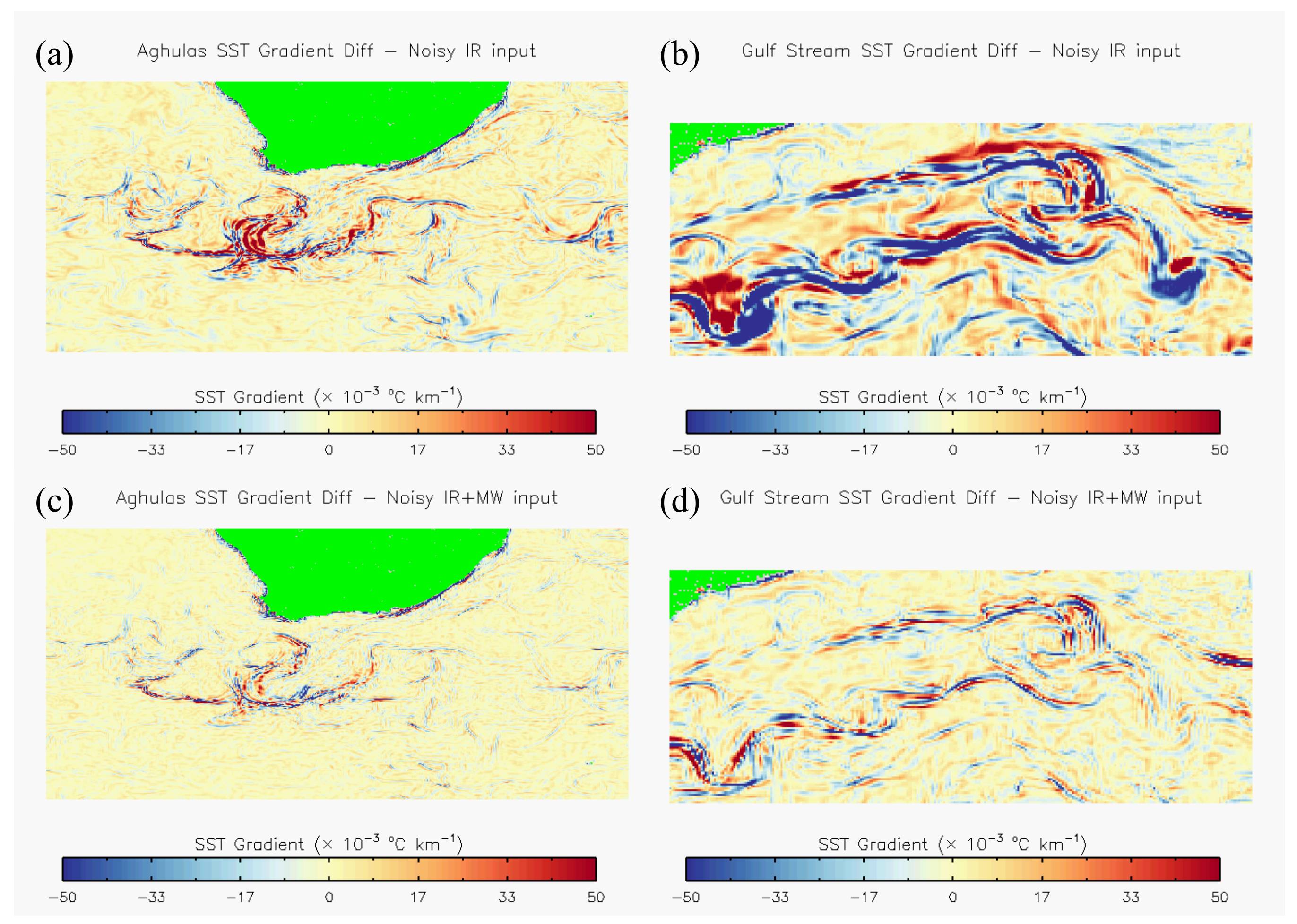
3.2. Reconstruction in Dynamical Regions
3.3. Reconstruction of the Southern Ocean and Maritime Continent
3.4. Summary
4. Conclusions
Author Contributions
Funding
Acknowledgments
Conflicts of Interest
References
- Clayson, C.A.; Chen, A.D. Sensitivity of a coupled single-column model in the tropics to treatment of the interfacial parameterizations. J. Clim. 2002, 15, 1805–1831. [Google Scholar] [CrossRef]
- Webster, P.J.; Clayson, C.A.; Curry, J.A. Clouds, Radiation, and the Diurnal Cycle of Sea Surface Temperature in the Tropical Western Pacific. J. Clim. 1996, 9, 1712–1730. [Google Scholar] [CrossRef]
- Chelton, D.B. The Impact of SST Specification on ECMWF Surface Wind Stress Fields in the Eastern Tropical Pacific. J. Clim. 2005, 18, 530–550. [Google Scholar] [CrossRef] [Green Version]
- Donlon, C.; Robinson, I.; Casey, K.S.; Vazquez-Cuervo, J.; Armstrong, E.; Arino, O.; Gentemann, C.; May, D.; LeBorgne, P.; Piollé, J.; et al. The Global Ocean Data Assimilation Experiment High-resolution Sea Surface Temperature Pilot Project. Bull. Am. Meteorol. Soc. 2007, 88, 1197–1214. [Google Scholar] [CrossRef]
- Nielsen-Englyst, P.; Høyer, J.L.; Toudal Pedersen, L.; Gentemann, C.L.; Alerskans, E.; Block, T.; Donlon, C. Optimal Estimation of Sea Surface Temperature from AMSR-E. Remote Sens. 2018, 10. [Google Scholar] [CrossRef]
- Pearson, K.; Gentemann, C.; Kachi, M. Comparison of AMSR2 Sea Surface Temperature Retrievals with In-Situ Data; Group for High Resolution Sea Surface Temperature (ESA/ESTEC): Noordwijk, The Netherlands, 2015; pp. 74–80. [Google Scholar]
- Merchant, C.J.; Embury, O.; Bulgin, C.E.; Block, T.; Corlett, G.; Fiedler, E.; Good, S.A.; Mittaz, J.; Rayner, N.; Berry, N.A.; et al. Satellite-based time-series of sea-surface temperature since 1981 for climate applications. Nat. Sci. Data 2019, in press. [Google Scholar]
- EU Arctic Policy. Available online: https://eeas.europa.eu/arctic-policy/eu-arctic-policy_en (accessed on 11 June 2019).
- Donlon, C. Copernicus Imaging Microwave Radiometer (CIMR)—Mission Requirements Document; ESA-EOPSM-CIMR-MRD-3236; European Space Agency: Katwijk, The Netherlands, 5 March 2019. [Google Scholar]
- Donlon, C.J.; Martin, M.; Stark, J.; Roberts-Jones, J.; Fiedler, E.; Wimmer, W. The Operational Sea Surface Temperature and Sea Ice Analysis (OSTIA) system. Remote Sens. Environ. 2012, 116, 140–158. [Google Scholar] [CrossRef]
- Donlon, C. Proceedings from the Third GODAE High Resolution SST Pilot Project Workshop; Technical Report No. 16; International GHRSST-PP Project Office: Leicester, UK, 2003. [Google Scholar]
- Donlon, C.; Emery, B.; Kawamura, H.; Cummings, J.; Robinson, I.; LeBorgne, P.; May, D.; Minnett, P.; Barton, I.; Rayner, N.; et al. The Recommended GHRSST-PP Data Processing Specification GDS; Technical report No. 17; International GHRSST-PP Project Office: Leicester, UK, 26 March 2004. [Google Scholar]
- Mogensen, K.S.; Balmaseda, M.A.; Weaver, A. The NEMOVAR Ocean Data Assimilation System as Implemented in the ECMWF Ocean Analysis for System 4; Technical Report No. 668; European Centre for Medium Range Weather Forecasts: Reading, UK, 2012. [Google Scholar]
- Fiedler, E.K.; Mao, C.; Good, S.A.; Water, J.; Martin, M.J. Improvements to feature resolution in the OSTIA sea surface temperature analysis using the NEMOVAR assimilation scheme. Q. J. R. Meteorol. Soc. 2019. [Google Scholar] [CrossRef]
- The North Atlantic Climate System Integrated Study. Available online: http://acsis.ac.uk (accessed on 11 June 2019).
- Gurvan, M.; Romain, B.-B.; Bouttier, P.-A.; Bricaud, C.; Bruciaferri, D.; Calvert, D.; Chanut, J.; Clementi, E.; Coward, A.; Delrosso, D.; et al. NEMO Ocean Model. In Nemo Ocean Engine; Notes du Pôle de Modélisation de l’Institut Pierre-Simon Laplace (IPSL): Paris, France, 2017. [Google Scholar] [CrossRef]
- Madec, G.; Imbard, M. A global ocean mesh to overcome the North Pole singularity. Clim. Dyn. 1996, 12, 381–388. [Google Scholar] [CrossRef]
- ORCA Tripolar Grid. Available online: https://www.nemo-ocean.eu/doc/node108.html (accessed on 4 July 2019).
- Le Traon, P.Y.; Klein, P.; Hua, B.L.; Dibarboure, G. Do Altimeter Wavenumber Spectra Agree with the Interior or Surface Quasigeostrophic Theory? J. Phys. Oceanogr. 2008, 38, 1137–1142. [Google Scholar] [CrossRef]
- Isern-Fontanet, J.; Chapron, B.; Lapeyre, G.; Klein, P. Potential use of microwave sea surface temperatures for the estimation of ocean currents. Geophys. Res. Lett. 2006, 33. [Google Scholar] [CrossRef] [Green Version]
- Mackie, S.; Embury, O.; Old, C.; Merchant, C.J.; Francis, P. Generalized Bayesian cloud detection for satellite imagery. Part 1: Technique and validation for night-time imagery over land and sea. Int. J. Remote Sens. 2010, 31, 2573–2594. [Google Scholar] [CrossRef]
- Mackie, S.; Merchant, C.J.; Embury, O.; Francis, P. Generalized Bayesian cloud detection for satellite imagery. Part 2: Technique and validation for daytime imagery. Int. J. Remote Sens. 2010, 31, 2595–2621. [Google Scholar] [CrossRef]
- Merchant, C.J.; Embury, O.; Roberts-Jones, J.; Fiedler, E.; Bulgin, C.E.; Corlett, G.K.; Good, S.; McLaren, A.; Rayner, N.; Morak-Bozzo, S.; et al. Sea surface temperature datasets for climate applications from Phase 1 of the European Space Agency Climate Change Initiative (SST CCI). Geosci. Data J. 2014, 1, 179–191. [Google Scholar] [CrossRef]
- Copernicus Climate Change Service Dataset: Sea Surface Temperature Integrated Climate Data Record (ICDR) from the Advanced Very High Resolution Radiometer (AVHRR), Level 3C (L3C), version 2; Copernicus Climate Change Service: Brussels, Belgium, 2019.
- Climate Data Store. Available online: https://cds.climate.copernicus.eu/#!/home (accessed on 8 July 2019).
- Rayner, N.; Good, S.A.; Block, T.; Evadzi, P.; Embury, O. SST CCI Product User Guide; Met Office: Exeter, UK, 2019. [Google Scholar]
- Bulgin, C.E.; Embury, O.; Corlett, G.; Merchant, C.J. Independent uncertainty estimates for coefficient based sea surface temperature retrieval from the Along-Track Scanning Radiometer instruments. Remote Sens. Environ. 2016, 178, 213–222. [Google Scholar] [CrossRef] [Green Version]
- Kilic, L.; Prigent, C.; Aires, F.; Boutin, J.; Heygster, G.; Tonboe, R.T.; Roquet, H.; Jimenez, C.; Donlon, C. Expected Performances of the Copernicus Imaging Microwave Radiometer (CIMR) for an All-Weather and High Spatial Resolution Estimation of Ocean and Sea Ice Parameters. J. Geophys. Res. Oceans 2018, 123, 7564–7580. [Google Scholar] [CrossRef]
- Fiedler, E.K.; McLaren, A.; Banzon, V.; Brasnett, B.; Ishizaki, S.; Kennedy, J.; Rayner, N.; Roberts-Jones, J.; Corlett, G.; Merchant, C.J.; et al. Intercomparison of long-term sea surface temperature analyses using the GHRSST Multi-Product Ensemble (GMPE) system. Remote Sens. Environ. 2019, 222, 18–33. [Google Scholar] [CrossRef]
- Reynolds, R.W.; Smith, T.M.; Liu, C.; Chelton, D.B.; Casey, K.S.; Schlax, M.G. Daily High-Resolution-Blended Analyses for Sea Surface Temperature. J. Clim. 2007, 20, 5473–5496. [Google Scholar] [CrossRef]
- Reynolds, R.W.; Chelton, D.B.; Roberts-Jones, J.; Martin, M.J.; Menemenlis, D.; Merchant, C.J. Objective Determination of Feature Resolution in Two Sea Surface Temperature Analyses. J. Clim. 2013, 26, 2514–2533. [Google Scholar] [CrossRef] [Green Version]
- Liu, Y.; Weisberg, R.H.; Law, J.; Huang, B. Evaluation of Satellite-Derived SST Products in Identifying the Rapid Temperature Drop on the West Florida Shelf Associated with Hurricane Irma. Mar. Technol. Soc. J. 2018, 52, 43–50. [Google Scholar] [CrossRef]


| Channel (GHz) | Utotal | UNEΔT | Uorb-stab | Ulife-stab | Upl-cal |
|---|---|---|---|---|---|
| 1.41 | 0.5 | 0.3 | 0.2 | 0.2 | 0.2 |
| 6.9 | 0.4 | 0.2 | 0.1 | 0.2 | 0.2 |
| 10.65 | 0.45 | 0.3 | 0.1 | 0.2 | 0.2 |
| 18.7 | 0.6 | 0.4 | 0.2 | 0.2 | 0.2 |
| 36.5 | 0.8 | 0.7 | 0.2 | 0.2 | 0.2 |
| Configuration | Global | Aghulas Current | Gulf Stream | Maritime | Southern Ocean | Coast | |
|---|---|---|---|---|---|---|---|
| Jan | Perfect IR-only | 0.310 | 0.532 | 1.286 | 0.394 | 0.369 | 0.641 |
| Perfect IR + CIMR | 0.175 | 0.312 | 0.358 | 0.212 | 0.132 | 0.608 | |
| Realistic IR-only | 0.369 | 0.587 | 1.289 | 0.462 | 0.396 | 0.667 | |
| Realistic IR + CIMR | 0.210 | 0.337 | 0.386 | 0.233 | 0.169 | 0.622 | |
| July | Perfect IR-only | 0.338 | 0.325 | 0.410 | 0.236 | 0.493 | 0.981 |
| Perfect IR + CIMR | 0.225 | 0.159 | 0.258 | 0.159 | 0.078 | 0.969 | |
| Realistic IR-only | 0.395 | 0.384 | 0.506 | 0.335 | 0.496 | 0.995 | |
| Realistic IR + CIMR | 0.249 | 0.199 | 0.284 | 0.200 | 0.130 | 0.969 | |
© 2019 by the authors. Licensee MDPI, Basel, Switzerland. This article is an open access article distributed under the terms and conditions of the Creative Commons Attribution (CC BY) license (http://creativecommons.org/licenses/by/4.0/).
Share and Cite
Pearson, K.; Good, S.; Merchant, C.J.; Prigent, C.; Embury, O.; Donlon, C. Sea Surface Temperature in Global Analyses: Gains from the Copernicus Imaging Microwave Radiometer. Remote Sens. 2019, 11, 2362. https://doi.org/10.3390/rs11202362
Pearson K, Good S, Merchant CJ, Prigent C, Embury O, Donlon C. Sea Surface Temperature in Global Analyses: Gains from the Copernicus Imaging Microwave Radiometer. Remote Sensing. 2019; 11(20):2362. https://doi.org/10.3390/rs11202362
Chicago/Turabian StylePearson, Kevin, Simon Good, Christopher J. Merchant, Catherine Prigent, Owen Embury, and Craig Donlon. 2019. "Sea Surface Temperature in Global Analyses: Gains from the Copernicus Imaging Microwave Radiometer" Remote Sensing 11, no. 20: 2362. https://doi.org/10.3390/rs11202362